In this section, we will look at some examples of tasks you might want to perform that involve reading and writing geo-spatial data in both vector and raster format.
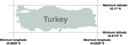
In this slightly contrived example, we will make use of a Shapefile to calculate the minimum and maximum latitude/longitude values for each country in the world. This "bounding box" can be used, among other things, to generate a map of a particular country. For example, the bounding box for Turkey would look like this:
Start by downloading the World Borders Dataset from:
http://thematicmapping.org/downloads/world_borders.php
Decompress the .zip archive and place the various files that make up the Shapefile (the .dbf, .prj, .shp, and .shx files) together in a suitable directory.
We next need to create a Python program that can read the borders of each country. Fortunately, using OGR to read through the contents of a Shapefile is trivial:
import osgeo.ogr

shapefile = osgeo.ogr.Open("TM_WORLD_BORDERS-0.3.shp")
layer = shapefile.GetLayer(0)

for i in range(layer.GetFeatureCount()):
    feature = layer.GetFeature(i)
The feature consists of a geometry and a set of fields. For this data, the geometry is a polygon that defines the outline of the country, while the fields contain various pieces of information about the country. According to the Readme.txt file, the fields in this Shapefile include the ISO-3166 three-letter code for the country (in a field named ISO3) as well as the name for the country (in a field named NAME). This allows us to obtain the country code and name like this:
countryCode = feature.GetField("ISO3")
countryName = feature.GetField("NAME")
We can also obtain the country's border polygon using:
geometry = feature.GetGeometryRef()
There are all sorts of things we can do with this geometry, but in this case we want to obtain the bounding box or envelope for the polygon:
minLong,maxLong,minLat,maxLat = geometry.GetEnvelope()
Let's put all this together into a complete working program:
# calcBoundingBoxes.py

import osgeo.ogr

shapefile = osgeo.ogr.Open("TM_WORLD_BORDERS-0.3.shp")
layer = shapefile.GetLayer(0)

countries = [] # List of (code,name,minLat,maxLat,
               # minLong,maxLong tuples.

for i in range(layer.GetFeatureCount()):
    feature = layer.GetFeature(i)
    countryCode = feature.GetField("ISO3")
    countryName = feature.GetField("NAME")
    geometry = feature.GetGeometryRef()
    minLong,maxLong,minLat,maxLat = geometry.GetEnvelope()

    countries.append((countryName, countryCode,
                      minLat, maxLat, minLong, maxLong))

countries.sort()
for name,code,minLat,maxLat,minLong,maxLong in countries:
    print "%s (%s) lat=%0.4f..%0.4f, long=%0.4f..%0.4f"
% (name, code,minLat, maxLat,minLong, maxLong)
Running this program produces the following output:
% python calcBoundingBoxes.py
Afghanistan (AFG) lat=29.4061..38.4721, long=60.5042..74.9157
Albania (ALB) lat=39.6447..42.6619, long=19.2825..21.0542
Algeria (DZA) lat=18.9764..37.0914, long=-8.6672..11.9865
...
While the previous example simply printed out the latitude and longitude values, it might be more useful to draw the bounding boxes onto a map. To do this, we have to convert the bounding boxes into polygons, and save these polygons into a Shapefile.
Creating a Shapefile involves the following steps:
- Define the spatial reference used by the Shapefile's data. In this case, we'll use the WGS84 datum and unprojected geographic coordinates (that is, latitude and longitude values). This is how you would define this spatial reference using OGR:
import osgeo.osr

spatialReference = osgeo.osr.SpatialReference()
spatialReference.SetWellKnownGeogCS('WGS84')
We can now create the Shapefile itself using this spatial reference:
import osgeo.ogr driver = osgeo.ogr.GetDriverByName("ESRI Shapefile") dstFile = driver.CreateDataSource(“boundingBoxes.shp")) dstLayer = dstFile.CreateLayer("layer", spatialReference) - After creating the Shapefile, you next define the various fields that will hold the metadata for each feature. In this case, let's add two fields to store the country name and its ISO-3166 code:
fieldDef = osgeo.ogr.FieldDefn("COUNTRY", osgeo.ogr.OFTString) fieldDef.SetWidth(50) dstLayer.CreateField(fieldDef) fieldDef = osgeo.ogr.FieldDefn("CODE", osgeo.ogr.OFTString) fieldDef.SetWidth(3) dstLayer.CreateField(fieldDef) - We now need to create the geometry for each feature—in this case, a polygon defining the country's bounding box. A polygon consists of one or more linear rings; the first linear ring defines the exterior of the polygon, while additional rings define "holes" inside the polygon. In this case, we want a simple polygon with a square exterior and no holes:
linearRing = osgeo.ogr.Geometry(osgeo.ogr.wkbLinearRing)
linearRing.AddPoint(minLong, minLat)
linearRing.AddPoint(maxLong, minLat)
linearRing.AddPoint(maxLong, maxLat)
linearRing.AddPoint(minLong, maxLat)
linearRing.AddPoint(minLong, minLat)

polygon = osgeo.ogr.Geometry(osgeo.ogr.wkbPolygon)
polygon.AddGeometry(linearRing)
Note
You may have noticed that the coordinate
(minLong, minLat)wasadded to the linear ring twice. This is because we are defining line segments rather than just points—the first call toAddPoint()definesthe starting point, and each subsequent call toAddPoint()addsa new line segment to the linear ring. In this case, we start in the lower-left corner and move counter-clockwise around the bounding box until we reach the lower-left corner again: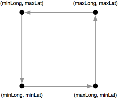
Once we have the polygon, we can use it to create a feature:
feature = osgeo.ogr.Feature(dstLayer.GetLayerDefn())
feature.SetGeometry(polygon)
feature.SetField("COUNTRY", countryName)
feature.SetField("CODE", countryCode)
dstLayer.CreateFeature(feature)
feature.Destroy()
Notice how we use the
setField()method to store the feature's metadata. We also have to call theDestroy()method to close the feature once we have finished with it; this ensures that the feature is saved into the Shapefile. - Finally, we call the
Destroy()method to close the output Shapefile:dstFile.Destroy()
- Putting all this together, and combining it with the code from the previous recipe to calculate the bounding boxes for each country in the World Borders Dataset Shapefile, we end up with the following complete program:
# boundingBoxesToShapefile.py

import os, os.path, shutil

import osgeo.ogr
import osgeo.osr

# Open the source shapefile.

srcFile = osgeo.ogr.Open("TM_WORLD_BORDERS-0.3.shp")
srcLayer = srcFile.GetLayer(0)

# Open the output shapefile.

if os.path.exists("bounding-boxes"):
    shutil.rmtree("bounding-boxes")
os.mkdir("bounding-boxes")

spatialReference = osgeo.osr.SpatialReference()
spatialReference.SetWellKnownGeogCS('WGS84')

driver = osgeo.ogr.GetDriverByName("ESRI Shapefile")
dstPath = os.path.join("bounding-boxes", "boundingBoxes.shp")
dstFile = driver.CreateDataSource(dstPath)
dstLayer = dstFile.CreateLayer("layer", spatialReference)

fieldDef = osgeo.ogr.FieldDefn("COUNTRY", osgeo.ogr.OFTString)
fieldDef.SetWidth(50)
dstLayer.CreateField(fieldDef)

fieldDef = osgeo.ogr.FieldDefn("CODE", osgeo.ogr.OFTString)
fieldDef.SetWidth(3)
dstLayer.CreateField(fieldDef)

# Read the country features from the source shapefile.

for i in range(srcLayer.GetFeatureCount()):
    feature = srcLayer.GetFeature(i)
countryCode = feature.GetField("ISO3")
    countryName = feature.GetField("NAME")
    geometry = feature.GetGeometryRef()
    minLong,maxLong,minLat,maxLat = geometry.GetEnvelope()

    # Save the bounding box as a feature in the output
    # shapefile.

    linearRing = osgeo.ogr.Geometry(osgeo.ogr.wkbLinearRing)
    linearRing.AddPoint(minLong, minLat)
    linearRing.AddPoint(maxLong, minLat)
    linearRing.AddPoint(maxLong, maxLat)
    linearRing.AddPoint(minLong, maxLat)
    linearRing.AddPoint(minLong, minLat)

    polygon = osgeo.ogr.Geometry(osgeo.ogr.wkbPolygon)
    polygon.AddGeometry(linearRing)

    feature = osgeo.ogr.Feature(dstLayer.GetLayerDefn())
    feature.SetGeometry(polygon)
feature.SetField("COUNTRY", countryName)
    feature.SetField("CODE", countryCode)
dstLayer.CreateFeature(feature)
    feature.Destroy()

# All done.

srcFile.Destroy()
dstFile.Destroy()
The only unexpected twist in this program is the use of a sub-directory called bounding-boxes to store the output Shapefile. Because a Shapefile is actually made up of multiple files on disk (a .dbf file, a .prj file, a .shp file, and a .shx file), it is easier to place these together in a sub-directory. We use the Python Standard Library module shutil to delete the previous contents of this directory, and then os.mkdir() to create it again.
Tip
If you aren't storing the TM_WORLD_BORDERS-0.3.shp Shapefile in the same directory as the script itself, you will need to add the directory where the Shapefile is stored to your osgeo.ogr.Open() call. You can also store the boundingBoxes.shp Shapefile in a different directory if you prefer, by changing the path where this Shapefile is created.
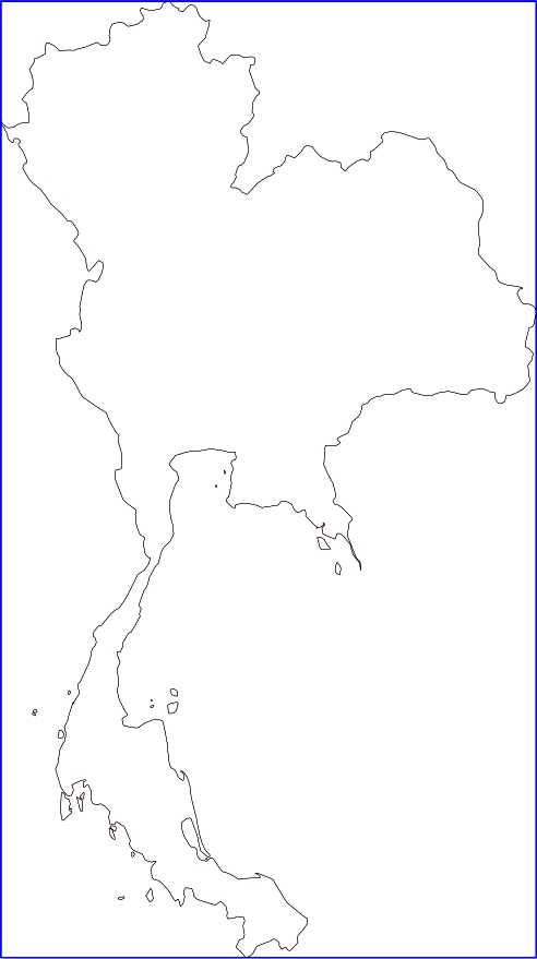
Running this program creates the bounding box Shapefile, which we can then draw onto a map. For example, here is the outline of Thailand along with a bounding box taken from the boundingBoxes.shp Shapefile:
We will be looking at how to draw maps in Chapter 8.
A DEM (Digital Elevation Map) is a type of raster format geo-spatial data where each pixel value represents the height of a point on the Earth's surface. We encountered DEM files in the previous chapter, where we saw two examples of datasources which supply this type of information: the National Elevation Dataset covering the United States, and GLOBE which provides DEM files covering the entire Earth.
Because a DEM file contains height data, it can be interesting to analyze the height values for a given area. For example, we could draw a histogram showing how much of a country's area is at a certain elevation. Let's take some DEM data from the GLOBE dataset, and calculate a height histogram using that data.
To keep things simple, we will choose a small country surrounded by the ocean: New Zealand.
Note
We're using a small country so that we don't have too much data to work with, and we're using a country surrounded by ocean so that we can check all the points within a bounding box rather than having to use a polygon to exclude points outside of the country's boundaries.
To download the DEM data, go to the GLOBE website (http://www.ngdc.noaa.gov/mgg/topo/globe.html) and click on the Get Data Online hyperlink. We're going to use the data already calculated for this area of the world, so click on the Any or all 16 "tiles" hyperlink. New Zealand is in tile L, so click on this tile to download it.
The file you download will be called l10g.gz. If you decompress it, you will end up with a file l10g containing the raw elevation data.
By itself, this file isn't very useful—it needs to be georeferenced onto the Earth's surface so that you can match up a height value with its position on the Earth. To do this, you need to download the associated header file. Unfortunately, the GLOBE website makes this rather difficult; the header files for the premade tiles can be found at:
http://www.ngdc.noaa.gov/mgg/topo/elev/esri/hdr
Download the file named l10g.hdr and place it into the same directory as the l10g file you downloaded earlier. You can then read the DEM file using GDAL:
import osgeo.gdal

dataset = osgeo.gdal.Open("l10g")
As you no doubt noticed when you downloaded the l10g tile, this covers much more than just New Zealand—all of Australia is included, as well as Malaysia, Papua New Guinea, and several other east-Asian countries. To work with the height data for just New Zealand, we have to be able to identify the relevant portion of the raster DEM—that is, the range of x,y coordinates which cover New Zealand. We start by looking at a map and identifying the minimum and maximum latitude/longitude values which enclose all of New Zealand, but no other country:
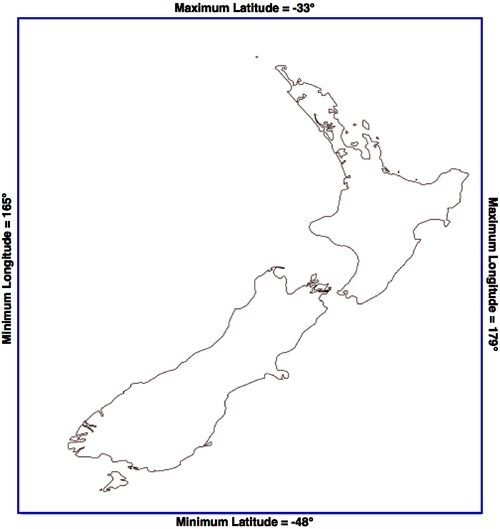
Rounded to the nearest whole degree, we get a long/lat bounding box of (165, -48)…(179, -33). This is the area we want to scan to cover all of New Zealand.
There is, however, a problem—the raster data consists of pixels or "cells" identified by (x,y) coordinates, not longitude and latitude values. We have to convert from longitudes and latitudes into x and y coordinates. To do this, we need to make use of the raster DEM's affine transformation.
If you can remember back to Chapter 3, an affine transformation is a set of six numbers that define how geographic coordinates (latitude and longitude values) are translated into raster (x,y) coordinates. This is done using two formulas:
longitude = t[0] + x*t[1] + y*t[2]
latitude = t[3] + x*t[4] + y*t[5]
Fortunately, we don't have to deal with these formulas directly as GDAL will do it for us. We start by obtaining our dataset's affine transformation:
t = dataset.GetGeoTransform()
Using this transformation, we could convert an x,y coordinate into its associated latitude and longitude value. In this case, however, we want to do the opposite—we want to take a latitude and longitude, and calculate the associated x,y coordinate.
To do this, we have to invert the affine transformation. Once again, GDAL will do this for us:
success,tInverse = gdal.InvGeoTransform(t)
if not success:
    print "Failed!"
    sys.exit(1)
Tip
There are some cases where an affine transformation can't be inverted. This is why gdal.InvGeoTransform() returns a success flag as well as the inverted transformation. With this DEM data, however, the affine transformation should always be invertible.
Now that we have the inverse affine transformation, it is possible to convert from a latitude and longitude into an x,y coordinate by using:
x,y = gdal.ApplyGeoTransform(tInverse, longitude, latitude)
Using this, it's easy to identify the minimum and maximum x,y coordinates that cover the area we are interested in:
x1,y1 = gdal.ApplyGeoTransform(tInverse, minLong, minLat)
x2,y2 = gdal.ApplyGeoTransform(tInverse, maxLong, maxLat)

minX = int(min(x1, x2))
maxX = int(max(x1, x2))
minY = int(min(y1, y2))
maxY = int(max(y1, y2))
Now that we know the x,y coordinates for the portion of the DEM that we're interested in, we can use GDAL to read in the individual height values. We start by obtaining the raster band that contains the DEM data:
band = dataset.GetRasterBand(1)
Now that we have the raster band, we can use the band.ReadRaster() method to read the raw DEM data. This is what the ReadRaster() method looks like:
ReadRaster(x, y, width, height, dWidth, dHeight, pixelType)
Where:
xis the number of pixels from the left side of the raster band to the left side of the portion of the band to read fromyis the number of pixels from the top of the raster band to the top of the portion of the band to read fromwidthis the number of pixels across to readheightis the number of pixels down to readdWidthis the width of the resulting datadHeightis the height of the resulting datapixelTypeis a constant defining how many bytes of data there are for each pixel value, and how that data is to be interpreted
Tip
Normally, you would set dWidth and dHeight to the same value as width and height; if you don't do this, the raster data will be scaled up or down when it is read.
The ReadRaster() method returns a string containing the raster data as a raw sequence of bytes. You can then read the individual values from this string using the struct standard library module:
values = struct.unpack("<" + ("h" * width), data)
Putting all this together, we can use GDAL to open the raster datafile and read all the pixel values within the bounding box surrounding New Zealand:
import sys, struct
from osgeo import gdal
from osgeo import gdalconst

minLat  = -48
maxLat  = -33
minLong = 165
maxLong = 179

dataset = gdal.Open("l10g")
band = dataset.GetRasterBand(1)

t = dataset.GetGeoTransform()
success,tInverse = gdal.InvGeoTransform(t)
if not success:
    print "Failed!"
    sys.exit(1)

x1,y1 = gdal.ApplyGeoTransform(tInverse, minLong, minLat)
x2,y2 = gdal.ApplyGeoTransform(tInverse, maxLong, maxLat)

minX = int(min(x1, x2))
maxX = int(max(x1, x2))
minY = int(min(y1, y2))
maxY = int(max(y1, y2))

width = (maxX - minX) + 1
fmt = "<" + ("h" * width)

for y in range(minY, maxY+1):
    scanline = band.ReadRaster(minX, y,width, 1,
                               width, 1,
                               gdalconst.GDT_Int16)
    values = struct.unpack(fmt, scanline)

    for value in values:
        ...
Tip
Don't forget to add a directory path to the gdal.Open()statement if you placed the l10g file in a different directory.
Let's replace the ... with some code that does something useful with the pixel values. We will calculate a histogram:
histogram = {} # Maps height to # pixels with that height.

...

for value in values:
    try:
        histogram[value] += 1
    except KeyError:
        histogram[value = 1

for height in sorted(histogram.keys()):
    print height,histogram[height]
If you run this, you will see a list of heights (in meters) and how many pixels there are at that height:
-
-500 2607581
1 6641
2 909
3 1628
...
3097 1
3119 2
3173 1
This reveals one final problem—there are a large number of pixels with a value of -500. What is going on here? Clearly -500 is not a valid height value. The GLOBE documentation explains:
Every tile contains values of -500 for oceans, with no values between -500 and the minimum value for land noted here.
So, all those points with a value of -500 represents pixels over the ocean. Fortunately, it is easy to exclude these; every raster file includes the concept of a no data value that is used for pixels without valid data. GDAL includes the GetNoDataValue() method that allows us to exclude these pixels:
for value in values:
    if value != band.GetNoDataValue():
        try:
            histogram[value] += 1
        except KeyError:
            histogram[value] = 1
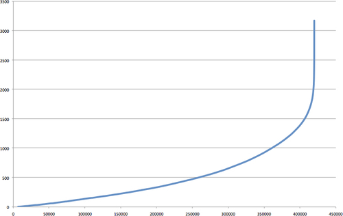
This finally gives us a histogram of the heights across New Zealand. You could create a graph using this data if you wished. For example, the following chart shows the total number of pixels at or below a given height: