
If you can remember from Chapter 2, a datum is a mathematical model of the Earth's shape, while a projection is a way of translating points on the Earth's surface into points on a two-dimensional map. There are a large number of available datums and projections—whenever you are working with geo-spatial data, you must know which datum and which projection (if any) your data uses. If you are combining data from multiple sources, you will often have to change your geo-spatial data from one datum to another, or from one projection to another.
Here, we will work with two Shapefiles that have different projections. We haven't yet encountered any geo-spatial data that uses a projection—all the data we've seen so far uses geographic (unprojected) latitude and longitude values. So, let's start by downloading some geo-spatial data in UTM (Universal Transverse Mercator) projection.
The WebGIS website (http://webgis.com) provides Shapefiles describing land-use and land-cover, called LULC datafiles. For this example, we will download a Shapefile for southern Florida (Dade County, to be exact) which uses the Universal Transverse Mercator projection.
You can download this Shapefile from the following URL:
http://webgis.com/MAPS/fl/lulcutm/miami.zip
The uncompressed directory contains the Shapefile, called miami.shp, along with a datum_reference.txt file describing the Shapefile's coordinate system. This file tells us the following:
The LULC shape file was generated from the original USGS GIRAS LULC file by Lakes Environmental Software.
Datum: NAD83
Projection: UTM
Zone: 17
Data collection date by U.S.G.S.: 1972
Reference: http://edcwww.cr.usgs.gov/products/landcover/lulc.html
So, this particular Shapefile uses UTM Zone 17 projection, and a datum of NAD83.
Let's take a second Shapefile, this time in geographic coordinates. We'll use the GSHHS shoreline database, which uses the WGS84 datum and geographic (latitude/longitude) coordinates.
Tip
You don't need to download the GSHHS database for this example; while we will display a map overlaying the LULC data over the top of the GSHHS data, you only need the LULC Shapefile to complete this recipe. Drawing maps such as the one shown below will be covered in Chapter 8.
Combining these two Shapefiles as they are would be impossible—the LULC Shapefile has coordinates measured in UTM (that is, in meters from a given reference line), while the GSHHS Shapefile has coordinates in latitude and longitude values (in decimal degrees):
LULC:  x=485719.47, y=2783420.62
       x=485779.49,y=2783380.63
       x=486129.65, y=2783010.66
       ...

GSHHS: x=180.0000,y=68.9938
       x=180.0000,y=65.0338
       x=179.9984, y=65.0337
       ...
Before we can combine these two Shapefiles, we first have to convert them to use the same projection. We'll do this by converting the LULC Shapefile from UTM-17 to geographic projection. Doing this requires us to define a coordinate transformation and then apply that transformation to each of the features in the Shapefile.
Here is how you can define a coordinate transformation using OGR:
from osgeo import osr

srcProjection = osr.SpatialReference()
srcProjection.SetUTM(17)

dstProjection = osr.SpatialReference()
dstProjection.SetWellKnownGeogCS('WGS84') # Lat/long.

transform = osr.CoordinateTransformation(srcProjection,
                                         dstProjection)
Using this transformation, we can transform each of the features in the Shapefile from UTM projection back into geographic coordinates:
for i in range(layer.GetFeatureCount()):
    feature = layer.GetFeature(i)
    geometry = feature.GetGeometryRef()
    geometry.Transform(transform)
    ...
Putting all this together with the techniques we explored earlier for copying the features from one Shapefile to another, we end up with the following complete program:
# changeProjection.py

import os, os.path, shutil
from osgeo import ogr
from osgeo import osr
from osgeo import gdal

# Define the source and destination projections, and a
# transformation object to convert from one to the other.

srcProjection = osr.SpatialReference()
srcProjection.SetUTM(17)

dstProjection = osr.SpatialReference()
dstProjection.SetWellKnownGeogCS('WGS84') # Lat/long.

transform = osr.CoordinateTransformation(srcProjection,
                                         dstProjection)

# Open the source shapefile.

srcFile = ogr.Open("miami/miami.shp")
srcLayer = srcFile.GetLayer(0)

# Create the dest shapefile, and give it the new projection.

if os.path.exists("miami-reprojected"):
    shutil.rmtree("miami-reprojected")
os.mkdir("miami-reprojected")

driver = ogr.GetDriverByName("ESRI Shapefile")
dstPath = os.path.join("miami-reprojected", "miami.shp")
dstFile = driver.CreateDataSource(dstPath)
dstLayer = dstFile.CreateLayer("layer", dstProjection)

# Reproject each feature in turn.

for i in range(srcLayer.GetFeatureCount()):
    feature = srcLayer.GetFeature(i)
    geometry = feature.GetGeometryRef()

    newGeometry = geometry.Clone()
    newGeometry.Transform(transform)

    feature = ogr.Feature(dstLayer.GetLayerDefn())
    feature.SetGeometry(newGeometry)
    dstLayer.CreateFeature(feature)
    feature.Destroy()

# All done.

srcFile.Destroy()
dstFile.Destroy()
Note
Note that this example doesn't copy field values into the new Shapefile; if your Shapefile has metadata, you will want to copy the fields across as you create each new feature. Also, the above code assumes that the miami.shp Shapefile has been placed into a miami sub-directory; you'll need to change the ogr.Open() statement to use the appropriate path name if you've stored this Shapefile in a different place.
After running this program over the miami.shp Shapefile, the coordinates for all the features in the Shapefile will have been converted from UTM-17 into geographic coordinates:
Before reprojection:  x=485719.47, y=2783420.62
                      x=485779.49,y=2783380.63
                      x=486129.65, y=2783010.66
                      ...

  After reprojection: x=-81.1417,y=25.1668
                      x=-81.1411,y=25.1664
                      x=-81.1376, y=25.1631
                      ...
To see that this worked, let's draw a map showing the reprojected LULC data on top of the GSHHS shoreline database:
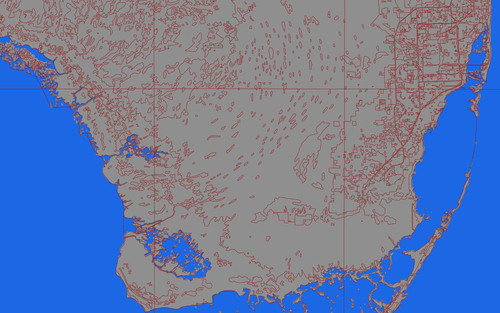
Both Shapefiles now use geographic coordinates, and as you can see the coastlines match exactly.
For this example, we will need to obtain some geo-spatial data that uses the NAD27 datum. This datum dates back to 1927, and was commonly used for North American geo-spatial analysis up until the 1980s when it was replaced by NAD83.
ESRI makes available a set of TIGER/Line files from the 2000 US census, converted into Shapefile format. These files can be downloaded from:
http://esri.com/data/download/census2000-tigerline/index.html
For the 2000 census data, the TIGER/Line files were all in NAD83 with the exception of Alaska, which used the older NAD27 datum. So, we can use this site to download a Shapefile containing features in NAD27. Go to the above site, click on the Preview and Download hyperlink, and then choose Alaska from the drop-down menu. Select the Line Features - Roads layer, then click on the Submit Selection button.
This data is divided up into individual counties. Click on the checkbox beside Anchorage, then click on the Proceed to Download button to download the Shapefile containing road details in Anchorage. The resulting Shapefile will be named tgr02020lkA.shp, and will be in a directory called lkA02020.
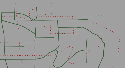
As described on the website, this data uses the NAD27 datum. If we were to assume this Shapefile used the WSG83 datum, all the features would be in the wrong place:

The heavy lines indicate where the features would appear if they were plotted using the incorrect WGS84 datum, while the thin dashed lines show where the features should really appear.
To make the features appear in the correct place, and to be able to combine these features with other features that use the WGS84 datum, we need to convert the Shapefile to use WGS84. Changing a Shapefile from one datum to another requires the same basic process we used earlier to change a Shapefile from one projection to another: first, you choose the source and destination datums, and define a coordinate transformation to convert from one to the other:
srcDatum = osr.SpatialReference()
srcDatum.SetWellKnownGeogCS('NAD27')

dstDatum = osr.SpatialReference()
dstDatum.SetWellKnownGeogCS('WGS84')

transform = osr.CoordinateTransformation(srcDatum, dstDatum)
You then process each feature in the Shapefile, transforming the feature's geometry using the coordinate transformation:
for i in range(srcLayer.GetFeatureCount()):
    feature = srcLayer.GetFeature(i)
    geometry = feature.GetGeometryRef()
    geometry.Transform(transform)
    ...
Here is the complete Python program to convert the lkA02020 Shapefile from the NAD27 datum to WGS84:
# changeDatum.py

import os, os.path, shutil
from osgeo import ogr
from osgeo import osr
from osgeo import gdal

# Define the source and destination datums, and a
# transformation object to convert from one to the other.

srcDatum = osr.SpatialReference()
srcDatum.SetWellKnownGeogCS('NAD27')

dstDatum = osr.SpatialReference()
dstDatum.SetWellKnownGeogCS('WGS84')

transform = osr.CoordinateTransformation(srcDatum, dstDatum)

# Open the source shapefile.

srcFile = ogr.Open("lkA02020/tgr02020lkA.shp")
srcLayer = srcFile.GetLayer(0)

# Create the dest shapefile, and give it the new projection.

if os.path.exists("lkA-reprojected"):
    shutil.rmtree("lkA-reprojected")
os.mkdir("lkA-reprojected")

driver = ogr.GetDriverByName("ESRI Shapefile")
dstPath = os.path.join("lkA-reprojected", "lkA02020.shp")
dstFile = driver.CreateDataSource(dstPath)
dstLayer = dstFile.CreateLayer("layer", dstDatum)

# Reproject each feature in turn.

for i in range(srcLayer.GetFeatureCount()):
    feature = srcLayer.GetFeature(i)
    geometry = feature.GetGeometryRef()

    newGeometry = geometry.Clone()
    newGeometry.Transform(transform)

    feature = ogr.Feature(dstLayer.GetLayerDefn())
    feature.SetGeometry(newGeometry)
    dstLayer.CreateFeature(feature)
    feature.Destroy()

# All done.

srcFile.Destroy()
dstFile.Destroy()
Tip
The above code assumes that the lkA02020 folder is in the same directory as the Python script itself. If you've placed this folder somewhere else, you'll need to change the ogr.Open() statement to use the appropriate directory path.
If we now plot the reprojected features using the WGS84 datum, the features will appear in the correct place:
The thin dashed lines indicate where the original projection would have placed the features, while the heavy lines show the correct positions using the reprojected data.