Let us now get started on the backpropagation algorithm:

1. Import the modules:

import tensorflow as tf 
from tensorflow.examples.tutorials.mnist import input_data 

2. Load the dataset; we use one-hot encoded labels by setting one_hot = True:

mnist = input_data.read_data_sets("MNIST_data/", one_hot=True) 
 

3. Define hyperparameters and other constants. Here, each handwritten digit is of the size 28 x 28 = 784 pixels. The dataset is classified into 10 categories, as digits can be any number between 0 to 9. These two are fixed. The learning rate, the maximum number of epochs, the batch size of the mini batch to be trained, and the number of neurons in the hidden layer are the hyperparameters. One can play around with them to see how they affect the network behaviour:

# Data specific constants
 n_input = 784 # MNIST data input (img shape: 28*28)
 n_classes = 10 # MNIST total classes (0-9 digits)

 # Hyperparameters
 max_epochs = 10000
 learning_rate = 0.5
 batch_size = 10
 seed = 0
 n_hidden = 30  # Number of neurons in the hidden layer 
 

4. We will require the derivative of the sigmoid function for weight update, so we define it:

def sigmaprime(x):
     return tf.multiply(tf.sigmoid(x), tf.subtract(tf.constant(1.0), tf.sigmoid(x))) 

5. Create placeholders for the training data:

x_in = tf.placeholder(tf.float32, [None, n_input])
y = tf.placeholder(tf.float32, [None, n_classes])

6. Create the model:

def multilayer_perceptron(x, weights, biases):
     # Hidden layer with RELU activation
     h_layer_1 = tf.add(tf.matmul(x, weights['h1']), biases['h1'])
     out_layer_1 = tf.sigmoid(h_layer_1)
     # Output layer with linear activation
     h_out = tf.matmul(out_layer_1, weights['out']) + biases['out']
     return tf.sigmoid(h_out), h_out, out_layer_1, h_layer_1 

7. Define variables for weights and biases:

weights = {
     'h1': tf.Variable(tf.random_normal([n_input, n_hidden], seed = seed)),
     'out': tf.Variable(tf.random_normal([n_hidden, n_classes], seed = seed)) }

 biases = {
     'h1': tf.Variable(tf.random_normal([1, n_hidden], seed = seed)),
     'out': tf.Variable(tf.random_normal([1, n_classes], seed = seed))} 

8. Create the computation graph for the forward pass, error, gradient, and update calculations:

# Forward Pass
 y_hat, h_2, o_1, h_1 = multilayer_perceptron(x_in, weights, biases)

 # Error
 err = y_hat - y

 # Backward Pass
 delta_2 = tf.multiply(err, sigmaprime(h_2))
 delta_w_2 = tf.matmul(tf.transpose(o_1), delta_2)

 wtd_error = tf.matmul(delta_2, tf.transpose(weights['out']))
 delta_1 = tf.multiply(wtd_error, sigmaprime(h_1))
 delta_w_1 = tf.matmul(tf.transpose(x_in), delta_1)

 eta = tf.constant(learning_rate)

 # Update weights
 step = [
     tf.assign(weights['h1'],tf.subtract(weights['h1'], tf.multiply(eta, delta_w_1)))
   , tf.assign(biases['h1'],tf.subtract(biases['h1'], tf.multiply(eta, tf.reduce_mean(delta_1, axis=[0]))))
   , tf.assign(weights['out'], tf.subtract(weights['out'], tf.multiply(eta, delta_w_2)))
   , tf.assign(biases['out'], tf.subtract(biases['out'], tf.multiply(eta,tf.reduce_mean(delta_2, axis=[0]))))
 ] 

9. Define ops for accuracy:

acct_mat = tf.equal(tf.argmax(y_hat, 1), tf.argmax(y, 1))
accuracy = tf.reduce_sum(tf.cast(acct_mat, tf.float32)) 

10. Initialize the variables:

init = tf.global_variables_initializer() 

11. Execute the graph:

with tf.Session() as sess:
     sess.run(init)
     for epoch in range(max_epochs):
         batch_xs, batch_ys = mnist.train.next_batch(batch_size)
         sess.run(step, feed_dict = {x_in: batch_xs, y : batch_ys})
         if epoch % 1000 == 0:
             acc_test = sess.run(accuracy, feed_dict =
                        {x_in: mnist.test.images,
                         y : mnist.test.labels})
             acc_train = sess.run(accuracy, feed_dict=
             {x_in: mnist.train.images,
              y: mnist.train.labels})
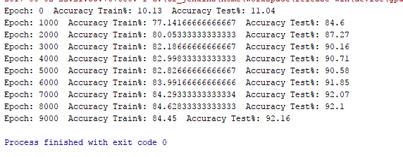
             print('Epoch: {0}  Accuracy Train%: {1}  Accuracy Test%: {2}'
                   .format(epoch,acc_train/600,(acc_test/100))) 

The result is as follows: