
Neural networks, also conventionally known as connectionist models, are inspired by the human brain. Like the human brain, neural networks are a collection of a large number of artificial neurons connected to each other via synaptic strengths called weights. Just as we learn through examples provided to us by our elders, artificial neural networks learn by examples presented to them as training datasets. With a sufficient number of training datasets, artificial neural networks can generalize the information and can then be employed for unseen data as well. Awesome, they sound like magic!
Neural networks are not new; the first neural network model, McCulloch Pitts (MCP) (http://vordenker.de/ggphilosophy/mcculloch_a-logical-calculus.pdf) Model, was proposed as early as 1943. (Yes, even before the first computer was built!) The model could perform logical operations like AND/OR/NOT. The MCP model had fixed weights and biases; there was no learning possible. This problem was resolved a few years later by Frank Rosenblatt in 1958 (https://blogs.umass.edu/brain-wars/files/2016/03/rosenblatt-1957.pdf). He proposed the first learning neural network called Perceptron.
From that time, it was known that adding multiple layers of neurons and building a deep and dense network will help neural networks solve complex tasks. Just as a mother is proud of her child's achievements, scientists and engineers made tall claims about what they can achieve using Neural Networks (NN) (https://www.youtube.com/watch?v=jPHUlQiwD9Y). The claims were not false, but it was simply not possible to accomplish them at that time because of the hardware computation limitation and complex network structure. This resulted in what is known as the AI Winters in the 1970s and 1980s; during these chills, the progress in this field slowed down due to very little or almost no funding to AI-based projects.
With the advent of DNNs and GPUs, the situation changed; today we have networks that can perform better with less tuning parameters, techniques like dropout and transfer learning the further reduce the training time, and lastly, the hardware companies that are coming up with specialized hardware chips to perform fast NN-based computations.
The artificial neuron is at the heart of all neural networks. It consists of two major components--an adder that (weighted) sums all the inputs to this neuron, and a processing unit that takes the weighted sum and generates an output based on a predefined function, called activation function. Each artificial neuron has its own set of weights and thresholds (biases); it learns these weights and thresholds through different learning algorithms:

Source: https://commons.wikimedia.org/wiki/File:Rosenblattperceptron.png
When only one layer of such neurons is present, it is called Perceptron. The input layer is called the zeroth layer as it simply buffers the input. The only layer of neurons present form the output layer. Each neuron of the output layer has its own weights and thresholds. When many such layers are present, the network is termed multi-layered perceptron (MLP). An MLP has one or more hidden layers. These hidden layers have a different number of hidden neurons. The neurons of each hidden layer have the same activation function:

The preceding figure shows an MLP with four inputs, five hidden layers, each with 4, 5, 6, 4, and 3 neurons respectively, and three neurons in the output layer. In MLP, all neurons of the lower layer are connected to all the neurons of the layer just above it. Therefore, MLPs are also called fully connected layers. The flow of information in MLPs is always from input to output; there are no feedback or jumps present, therefore these networks are also known as feedforward networks.
Perceptrons are trained using gradient descent algorithms. In Chapter 2, Regression, you learned about gradient descent; here we look at it a little deeper. Perceptrons learn through supervised learning algorithms, that is, the network is provided by the desired output for all the inputs present in the training dataset. At the output, we define an error function or objective function J(W), such that when the network has completely learned all the training data, the objective function will be minimum.
The weights of the output layer and the hidden layers are updated such that the gradient of the objective function decreases:
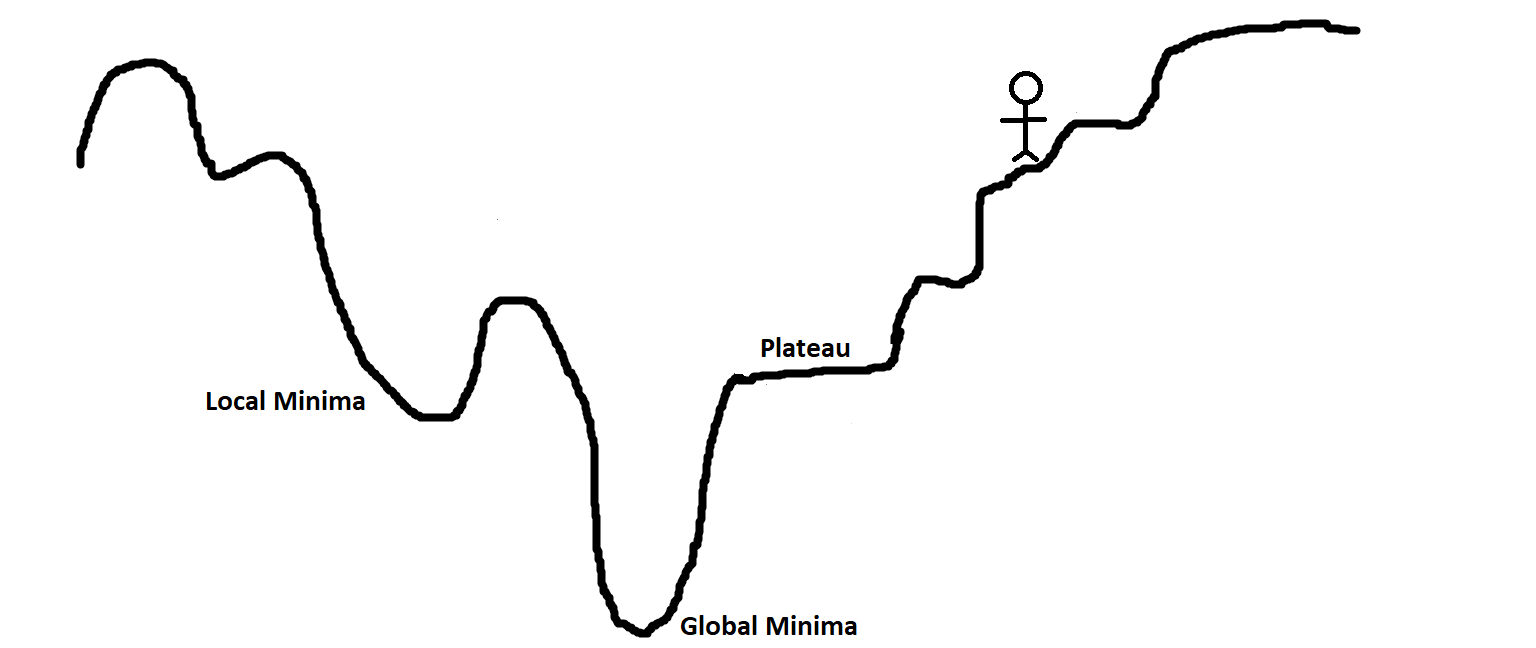
To understand it better, visualize a landscape full of hills, plateaus, and pits. The goal is to come to the ground (global minima of the objective function). If you are standing on top and you have to come down, it is an obvious choice that you will move down the hill, that is, toward the negative slope (or negative gradient). In the same manner, the weights in the Perceptron are changed proportionally to the negative of the gradient of the objective function.
The higher the value of the gradient, the larger will be the change in weight values and vice versa. Now, all this is quite fine, but we can land up with problems when we reach plateaus as the gradient is zero and hence there is no change in weights. We can also land in problems when we enter a small pit (local minima) because when we try to move to either side, the gradient will increase, forcing the network to stay in the pit.
As discussed in Chapter 2, Regression, there are various variants of gradient descent aimed at increasing convergence and that avoid the problem of getting stuck at local minima or plateaus (adding momentum, variable learning rate).
TensorFlow calculates these gradients automatically with the help of different optimizers. The important thing to note, however, is that as TensorFlow will calculate gradients, which will involve derivatives of the activation functions as well, it is important that the activation function you choose is differentiable and preferably has a non-zero gradient throughout the training scenario.
One of the major ways gradient descent for perceptrons differ from Chapter 2, Regression, applications is that the objective function is defined for the output layer, but is used to find the weight change of the neurons of the hidden layers as well. This is done using the backpropagation (BPN) algorithm, where the error at the output is propagated backwards to the hidden layers and used to determine the weight change. You will learn more about it soon.