
We proceed with the recipe as follows:
- Import matplotlib and the modules used by keras-vis. In addition, also import the pre-built VGG16 module. Keras makes it easy to deal with this pre-built network:
from matplotlib import pyplot as plt
from vis.utils import utils
from vis.utils.vggnet import VGG16
from vis.visualization import visualize_class_activation
- Access the VGG16 network by using the pre-built layers included in Keras and trained with ImageNet weights:
# Build the VGG16 network with ImageNet weights
model = VGG16(weights='imagenet', include_top=True)
model.summary()
print('Model loaded.')
- This is how the VGG16 network looks internally. We have many ConvNets, alternated with maxpool2D. Then, we have a Flatten layer followed by three Dense layers. The last one is called predictions, and this layer should be able to detect high-level features such as faces or, in our case, the shape of a bird. Note that the top layer is explicitly included in our network because we want to visualize what it learned:
_________________________________________________________________
 Layer (type) Output Shape Param #
 =================================================================
 input_2 (InputLayer) (None, 224, 224, 3) 0
 _________________________________________________________________
 block1_conv1 (Conv2D) (None, 224, 224, 64) 1792
 _________________________________________________________________
 block1_conv2 (Conv2D) (None, 224, 224, 64) 36928
 _________________________________________________________________
 block1_pool (MaxPooling2D) (None, 112, 112, 64) 0
 _________________________________________________________________
 block2_conv1 (Conv2D) (None, 112, 112, 128) 73856
 _________________________________________________________________
 block2_conv2 (Conv2D) (None, 112, 112, 128) 147584
 _________________________________________________________________
 block2_pool (MaxPooling2D) (None, 56, 56, 128) 0
 _________________________________________________________________
 block3_conv1 (Conv2D) (None, 56, 56, 256) 295168
 _________________________________________________________________
 block3_conv2 (Conv2D) (None, 56, 56, 256) 590080
 _________________________________________________________________
 block3_conv3 (Conv2D) (None, 56, 56, 256) 590080
 _________________________________________________________________
 block3_pool (MaxPooling2D) (None, 28, 28, 256) 0
 _________________________________________________________________
 block4_conv1 (Conv2D) (None, 28, 28, 512) 1180160
 _________________________________________________________________
 block4_conv2 (Conv2D) (None, 28, 28, 512) 2359808
 _________________________________________________________________
 block4_conv3 (Conv2D) (None, 28, 28, 512) 2359808
 _________________________________________________________________
 block4_pool (MaxPooling2D) (None, 14, 14, 512) 0
 _________________________________________________________________
 block5_conv1 (Conv2D) (None, 14, 14, 512) 2359808
 _________________________________________________________________
 block5_conv2 (Conv2D) (None, 14, 14, 512) 2359808
 _________________________________________________________________
 block5_conv3 (Conv2D) (None, 14, 14, 512) 2359808
 _________________________________________________________________
 block5_pool (MaxPooling2D) (None, 7, 7, 512) 0
 _________________________________________________________________
 flatten (Flatten) (None, 25088) 0
 _________________________________________________________________
 fc1 (Dense) (None, 4096) 102764544
 _________________________________________________________________
 fc2 (Dense) (None, 4096) 16781312
 _________________________________________________________________
 predictions (Dense) (None, 1000) 4097000
 =================================================================
 Total params: 138,357,544
 Trainable params: 138,357,544
 Non-trainable params: 0
 _________________________________________________________________
 Model loaded.
Visually, the network can be represented as shown in the following figure:
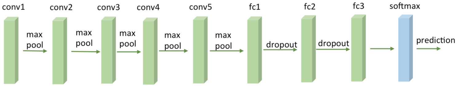
A VGG16 Network
- Now let's focus on inspecting how the last prediction layer looks internally by focusing on American Dipper, which is the ID 20:
layer_name = 'predictions'
layer_idx = [idx for idx, layer in enumerate(model.layers) if layer.name == layer_name][0]
# Generate three different images of the same output index.
vis_images = []
for idx in [20, 20, 20]:
img = visualize_class_activation(model, layer_idx, filter_indices=idx, max_iter=500)
img = utils.draw_text(img, str(idx))
vis_images.append(img)
- Let's display the generated images for the specific layer given the features and observe how the concept of the American Dipper bird is internally seen by the network:
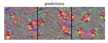
So, this is how a bird is internally represented by a neural network. It is a kind of trippy image, but I swear that no particular kind of artificial drug has been given to the network itself! This is just what this particular kind of artificial network has naturally learned.
- Are you are still curious to understand a bit more? Well, let's pick an earlier layer and represent how the network is internally seeing this same American Dipper training class:
layer_name = 'block3_conv1'
layer_idx = [idx for idx, layer in enumerate(model.layers) if layer.name == layer_name][0]
vis_images = []
for idx in [20, 20, 20]:
img = visualize_class_activation(model, layer_idx, filter_indices=idx, max_iter=500)
img = utils.draw_text(img, str(idx))
vis_images.append(img)
stitched = utils.stitch_images(vis_images)
plt.axis('off')
plt.imshow(stitched)
plt.title(layer_name)
plt.show()
The following is the output of the preceding code:
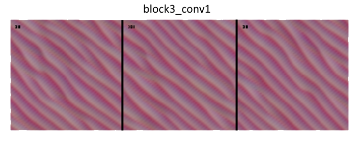
As expected, this particular layer is learning very basic features such as curves. However, the true power of ConvNets is that the network infers more and more sophisticated features the deeper we go into the models.