We proceed with the recipe as follows:

1. Install NSynth by creating a separate conda environment. Create and activate a Magenta conda environment using Python 2.7 with Jupyter Notebook support:

conda create -n magenta python=2.7 jupyter
source activate magenta

2. Install the Magenta pip package and the librosa, which is used for reading audio formats:

pip install magenta
pip install librosa

3. Install a pre-built model from the internet http://download.magenta.tensorflow.org/models/nsynth/wavenet-ckpt.tar and download a sample sound https://www.freesound.org/people/MustardPlug/sounds/395058/. Then run the notebook contained in the demo directory (in my case http://localhost:8888/notebooks/nsynth/Exploring_Neural_Audio_Synthesis_with_NSynth.ipynb) . The first part is about including modules that will be used later in our computations:

import os
import numpy as np
import matplotlib.pyplot as plt
from magenta.models.nsynth import utils
from magenta.models.nsynth.wavenet import fastgen
from IPython.display import Audio
%matplotlib inline
%config InlineBackend.figure_format = 'jpg'

4. Then we load the demo sound downloaded from the internet and put it in the same directory as the notebook. This will load 40,000 samples in about 2.5 seconds into the machine:

# from https://www.freesound.org/people/MustardPlug/sounds/395058/
fname = '395058__mustardplug__breakbeat-hiphop-a4-4bar-96bpm.wav'
sr = 16000
audio = utils.load_audio(fname, sample_length=40000, sr=sr)
sample_length = audio.shape[0]
print('{} samples, {} seconds'.format(sample_length, sample_length / float(sr)))

5. The next step is to encode the audio samples in a very compact representation using a pre-trained NSynth model downloaded from the internet. This will give us a 78 x 16 dimension encoding for every four seconds of audio, which we can then decode or resynthesize. Our encoding is a tensor (#files=1 x 78 x 16):

%time encoding = fastgen.encode(audio, 'model.ckpt-200000', sample_length)
INFO:tensorflow:Restoring parameters from model.ckpt-200000
 CPU times: user 1min 4s, sys: 2.96 s, total: 1min 7s
 Wall time: 25.7 s
print(encoding.shape)
(1, 78, 16)

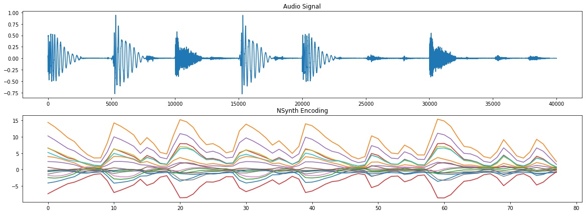
6. Let's save the encoding that will be used later for re-synthesizing. In addition, let's have a quick view of what the encoding shape is with a graphical representation and compare it with the original audio signal. As you can see, the encoding follows the beat presented in the original audio signal:

np.save(fname + '.npy', encoding)
fig, axs = plt.subplots(2, 1, figsize=(10, 5))
axs[0].plot(audio);
axs[0].set_title('Audio Signal')
axs[1].plot(encoding[0]);
axs[1].set_title('NSynth Encoding')

We observe the following audio signal and Nsynth Encoding:

7. Now let's do a decoding of the encoding we just produced. In other words, we try to reproduce the original audio from the compact representation with the intent of understanding if the re-synthesized sound is similar to the original one. Indeed, if you run the experiment and listen to the original audio and the re-synthesized one, they sound very similar:

%time fastgen.synthesize(encoding, save_paths=['gen_' + fname], samples_per_save=sample_length)