We proceed with the recipe as follows:
- As always, we start with importing the necessary modules:
import tensorflow as tf
import numpy as np
import matplotlib.pyplot as plt
%matplotlib inline
- Next, we declare a class, WTU, which will perform all the tasks. The class is instantiated with m x n the size of the 2D SOM lattice, dim the number of dimensions in the input data, and the total number of iterations:
def __init__(self, m, n, dim, num_iterations, eta = 0.5, sigma = None):
    """
    m x n : The dimension of 2D lattice in which neurons are     arranged
    dim : Dimension of input training data
    num_iterations: Total number of training iterations
    eta : Learning rate
    sigma: The radius of neighbourhood function.
    """
    self._m = m
    self._n = n
    self._neighbourhood = []
    self._topography = []
    self._num_iterations = int(num_iterations)
    self._learned = False
- In the __init__ itself, we define the computation graph and the session.
- If the network is not provided with any sigma value, it will take a default value, which is normally half of the maximum dimension of the SOM lattice:
if sigma is None:
    sigma = max(m,n)/2.0 # Constant radius
else:
    sigma = float(sigma)
- Next, in the graph, we declare variables for the weight matrix, placeholders for the input, and computational steps to calculate the winner and update its and its neighbors' weight. As SOM provides a topographic map, we also add ops to get the topographic location of neurons:
self._graph = tf.Graph()

# Build Computation Graph of SOM
 with self._graph.as_default():
# Weight Matrix and the topography of neurons
    self._W = tf.Variable(tf.random_normal([m*n, dim], seed = 0))
    self._topography = tf.constant(np.array(list(self._neuron_location(m, n))))

    # Placeholders for training data
    self._X = tf.placeholder('float', [dim])

    # Placeholder to keep track of number of iterations
    self._iter = tf.placeholder('float')

    # Finding the Winner and its location
    d = tf.sqrt(tf.reduce_sum(tf.pow(self._W - tf.stack([self._X
          for i in range(m*n)]),2),1))
    self.WTU_idx = tf.argmin(d,0)
    slice_start = tf.pad(tf.reshape(self.WTU_idx, [1]),np.array([[0,1]]))
    self.WTU_loc = tf.reshape(tf.slice(self._topography, slice_start,             [1,2]), [2])
    # Change learning rate and radius as a function of iterations
    learning_rate = 1 - self._iter/self._num_iterations
    _eta_new = eta * learning_rate
    _sigma_new = sigma * learning_rate

    # Calculating Neighbourhood function
    distance_square = tf.reduce_sum(tf.pow(tf.subtract(
    self._topography, tf.stack([self.WTU_loc for i in range(m * n)])), 2), 1)
    neighbourhood_func = tf.exp(tf.negative(tf.div(tf.cast(
distance_square, "float32"), tf.pow(_sigma_new, 2))))

    # multiply learning rate with neighbourhood func
    eta_into_Gamma = tf.multiply(_eta_new, neighbourhood_func)

    # Shape it so that it can be multiplied to calculate dW
    weight_multiplier = tf.stack([tf.tile(tf.slice(
eta_into_Gamma, np.array([i]), np.array([1])), [dim])
for i in range(m * n)])
    delta_W = tf.multiply(weight_multiplier,
tf.subtract(tf.stack([self._X for i in range(m * n)]),self._W))
    new_W = self._W + delta_W
    self._training = tf.assign(self._W,new_W)

   # Initialize All variables
   init = tf.global_variables_initializer()
   self._sess = tf.Session()
   self._sess.run(init)
- We define a fit method for the class, which executes the training op declared in the default graph of the class. The method also calculates centroid grid:
def fit(self, X):
 """
 Function to carry out training
 """
 for i in range(self._num_iterations):
   for x in X:
       self._sess.run(self._training, feed_dict= {self._X:x, self._iter: i})


 # Store a centroid grid for easy retreival
 centroid_grid = [[] for i in range(self._m)]
 self._Wts = list(self._sess.run(self._W))
 self._locations = list(self._sess.run(self._topography))
 for i, loc in enumerate(self._locations):
      centroid_grid[loc[0]].append(self._Wts[i])
 self._centroid_grid = centroid_grid

 self._learned = True
- We define a function to determine the index and the location of the winning neuron in the 2D lattice:
def winner(self, x):
    idx = self._sess.run([self.WTU_idx,self.WTU_loc], feed_dict = {self._X:x})
    return idx
- We define some more helper functions to perform the 2D mapping of neurons in the lattice and to map input vectors to the relevant neurons in the 2D lattice:
def _neuron_location(self,m,n):
    """
    Function to generate the 2D lattice of neurons
    """
    for i in range(m):
       for j in range(n):
           yield np.array([i,j])


def get_centroids(self):
    """
    Function to return a list of 'm' lists, with each inner     list containing the 'n' corresponding centroid locations     as 1-D NumPy arrays.
    """
    if not self._learned:
       raise ValueError("SOM not trained yet")
    return self._centroid_grid
def map_vects(self, X):
    """
    Function to map each input vector to the relevant neuron         in the lattice
    """
    if not self._learned:
        raise ValueError("SOM not trained yet")
    to_return = []
    for vect in X:
       min_index = min([i for i in range(len(self._Wts))],
       key=lambda x: np.linalg.norm(vect -
self._Wts[x]))
       to_return.append(self._locations[min_index])
return to_return
- Now that our WTU class is ready, we read data from the .csv file and normalize it:
def normalize(df):
    result = df.copy()
    for feature_name in df.columns:
       max_value = df[feature_name].max()
       min_value = df[feature_name].min()
       result[feature_name] = (df[feature_name] - min_value) / (max_value - min_value)
    return result

# Reading input data from file
import pandas as pd
df = pd.read_csv('colors.csv') # The last column of data file is a label
data = normalize(df[['R', 'G', 'B']]).values
name = df['Color-Name'].values
n_dim = len(df.columns) - 1

# Data for Training
colors = data
color_names = name
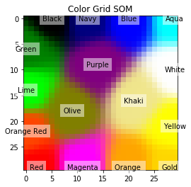
- Finally, we use our class to perform dimensionality reduction and arrange it in a beautiful topographic map:
som = WTU(30, 30, n_dim, 400, sigma=10.0)
som.fit(colors)

# Get output grid
image_grid = som.get_centroids()

# Map colours to their closest neurons
mapped = som.map_vects(colors)

# Plot
plt.imshow(image_grid)
plt.title('Color Grid SOM')
for i, m in enumerate(mapped):
     plt.text(m[1], m[0], color_names[i], ha='center', va='center', bbox=dict(facecolor='white', alpha=0.5, lw=0))
The plot is as follows: