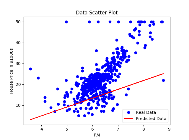
From the plot, we can see that our simple linear regressor tries to fit a linear line to the given dataset:

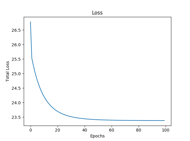
In the following graph, we can see that as our model learned the data, the loss function decreased, as was expected:

The following is the TensorBoard graph of our simple linear regressor:

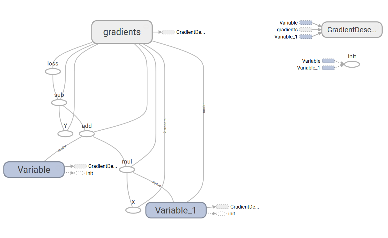
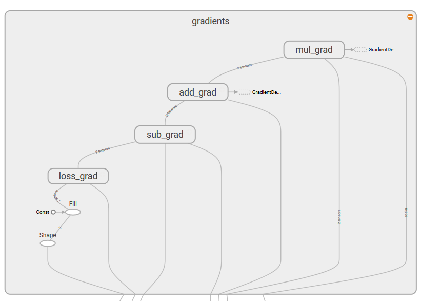
The graph has two name scope nodes, Variable and Variable_1, they are the high-level nodes representing bias and weights respectively. The node named gradient is also a high-level node; expanding the node, we can see that it takes seven inputs and computes the gradients that are then used by GradientDescentOptimizer to compute and apply updates to weights and bias: