
8.2 COMPARING DAG AND DCG ALGORITHMS
Figure 8.1a is an example of a DAG algorithm and Fig. 8.1b is an example of a DCG algorithm. An algorithm represented with a DAG requires a certain time to complete its tasks and the data flow is unidirectional from the inputs to the outputs. Thus, each task in the graph is completed once for each instance of the algorithm. When all tasks have been completed, the algorithm is terminated or another instance of it is started with another set of input data.
Figure 8.1 Example directed graphs for nonserial–parallel algorithms. (a) Directed acyclic graph (DAG). (b) Directed cyclic graph (DCG).
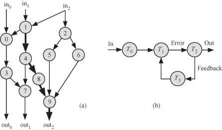
The DCG is most commonly encountered in discrete time feedback control systems such as adaptive filters and digital controllers for plant control. An example of a feedback control systems is a car automatic speed control and the airplane autopilot. The input is supplied to task T0 for prefiltering or for input signal conditioning. Task T1 accepts the conditioned input signal and the conditioned feedback output signal. The output of task T1 is usually referred to as the error signal, and this signal is fed to task T2 to produce the output signal. An algorithm represented by a DCG usually operates on a set of input data streams and produces a set of output data streams. The time between samples is called the sample time, which is equal to the maximum delay exhibited by any of the tasks shown in Fig. 8.1:
(8.1)
![]()
where τsample is the sample time and τi is the execution time of task Ti. This equation is similar to determining the pipeline period for a pipelined system as was discussed in Chapter 2. During each sample time, all the tasks must be evaluated. To shorten the sample time and to speed up the system data rate, we must shorten the execution times of each task individually. Table 8.1 compares the two main types of NSPAs: DAG and DCG. The techniques we use to accomplish this depend on the nature of the algorithms or functions implemented in each task. Thus, we can use techniques discussed in Chapters 2, 9–11, and 7 and in this chapter.
Table 8.1 Comparing the Two Main Types of NSPA Algorithms
| DAG | DCG |
| Algorithm parallelization attempts to determine which of the algorithm tasks can be executed at the same time. | Algorithm parallelization attempts to parallelize each task independently of the other tasks. |
| An algorithm instance executes once only. | An algorithm instance executes one for each sample time and repeats for as long as we have input data or for as long as we desire output data. |
| Input data are available initially before the algorithm is started. | Input data are supplied in a stream or as long as the algorithm is executing. |
| Output data are obtained typically after the algorithm has finished executing. | Output data are obtained in a stream as long as the algorithm is running. |
| The characteristic time is the algorithm execution time, which depends on the critical path. | The characteristic time is the sample time. |
| The workload is the number of tasks to be executed (W). | The workload is W for each sample time; that is, all tasks execute for each time step and then all of them are evaluated again at the next time step. |
| The application domain is typically abstract data fairly detached from actual physical phenomena. | The application domain is typically applied to tangible physical phenomena to be controlled, such as speed, temperature, pressure, and fluid flow. |