
Step 4: Interpret the Regression Slopes
Introduction to the Regression Parameters
To begin our discussion
on the regression line, let us start by looking at the “Parameter
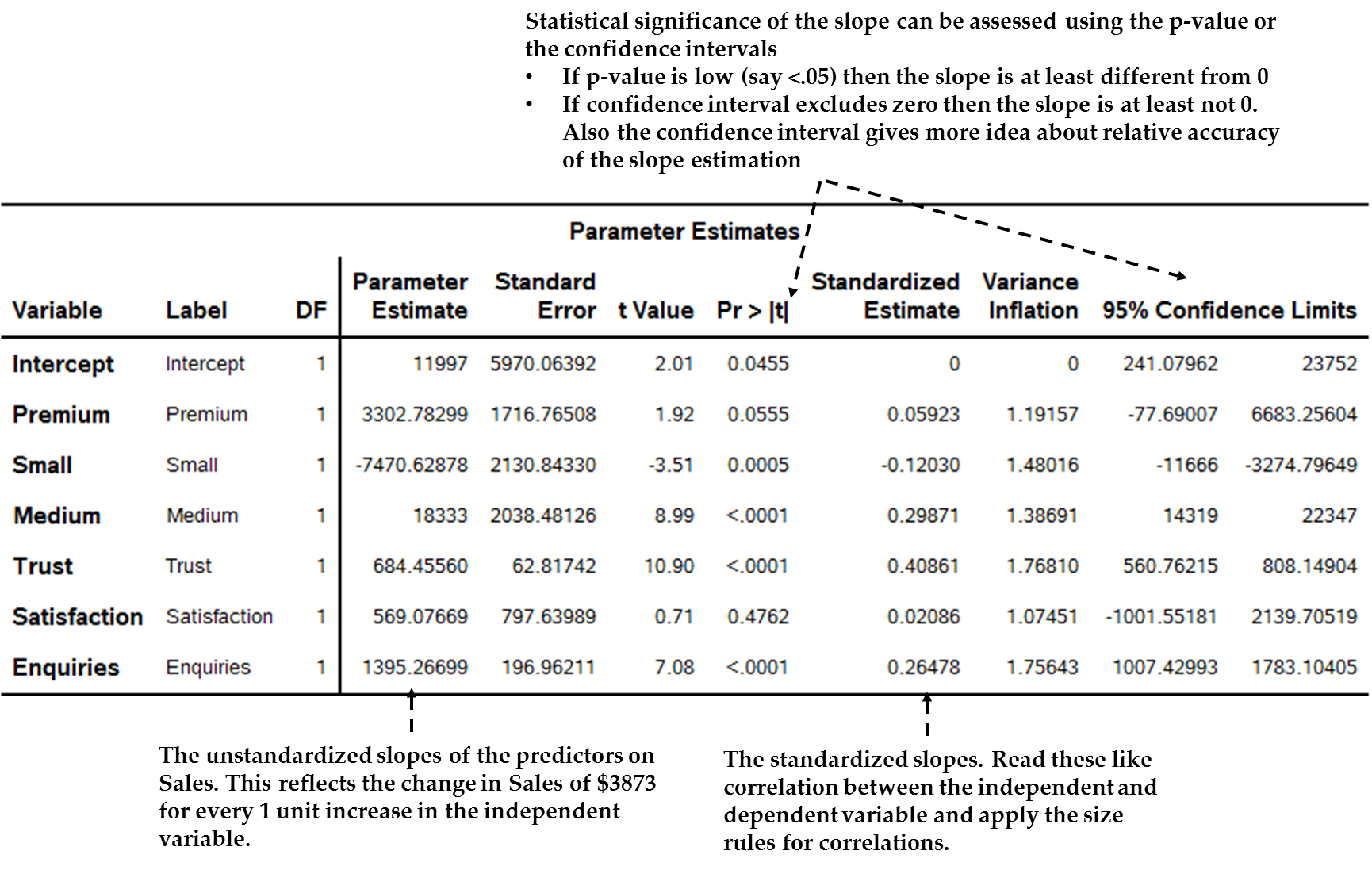
Estimates” table from our simple SAS example, as seen in Figure 13.27 The regression parameters table (slopes and intercept) in SAS below.
Figure 13.27 The regression parameters table (slopes and intercept) in SAS
We see rows for two
types of parameters in this table, one for the intercept and the rest
for the independent variable slopes. The following sections discuss
these two elements of the parameters table.
Regression Line Element #1: The Intercept
To begin, we say that,
without the independent variables, the best guess of the dependent
variable is probably its own mean. This average is not necessarily
a good guess (especially if the dependent variable is widely distributed),
but it is as good as you can do as a starting point.
To reflect the dependent
variable average, we usually include an intercept,
sometimes called the constant, which reflects the expected average
value of the dependent variable (e.g. “predicted sales”) if
the independent variables are all zero.
For example, in Figure 13.27 The regression parameters table (slopes and intercept) in SAS we see the intercept in the first row of the “Parameter
Estimate” column, with a value of 11997. In other words, when
a customer has zero enquiries, satisfaction, trust and so on, average
annual Sales are expected to be $11,997.
The intercept is often
not seen as important by analysts, especially when the independent
variable actually cannot have a zero, although there are cases when
it is a point of interest. In this case, it will not be of much interest
except perhaps as the starting point for the incremental value of
enquiries as discussed next.
There is one extra small
point to add about intercepts. If you know that the value of the dependent
variable should be zero when the independent variables are zero, then
you can and should ask SAS to force this fact into the analysis. Say,
for instance, that you wish to study the relationship between the
number of share trades on the stock exchange and the value of the
trades. If there are zero trades there must be zero value, and you
would include an extra keyword to reflect this.
Regression Line Element #2: Independent Variable Slopes
Introduction to Regression Slopes
In regression we analyze
independent variables in an attempt to gain better explanation of
the dependent variable than its own average. Slopes are the important
end outcome of a regression analysis. They reflect the strength of
the association and inferred causation between each independent variable
and the dependent variable. You can think of them as weights: if the
independent variable has any relationship with the dependent variable,
what is its strength? The slope reflects this.
As seen in Figure 13.27 The regression parameters table (slopes and intercept) in SAS, there are in fact two versions of the regression slope,
namely:
-
Unstandardized slopes: These are reflected in the “Parameter Estimate” column.
-
Standardized slopes: These are in the “Standardized Estimate” column.
In addition, as seen
in Figure 13.27 The regression parameters table (slopes and intercept) in SAS, there are two main measures of statistical significance
as discussed in Chapter 12, namely:
-
Confidence intervals: The last two columns of the Parameter Estimates table are 95% confidence intervals for the slope and intercept.
-
p-values: We see the p-values in the Pr > |t| column.
The next sections explain
these measures of statistical significance and the types of slopes,
after an initial process for how to approach the analysis of regression
parameters as a whole.
Process for Interpreting Regression Slopes
Figure 13.28 Interpreting regression-type slopes suggests a process for your overall analysis of regression
slopes.
Figure 13.28 Interpreting regression-type slopes

The following sections
unpack each of these steps.
Slope Assessment # 1: Significance and Accuracy of the Slope
As per the discussion
in Chapter 12, we often start by looking at the estimated accuracy
of statistics such as regression slopes, i.e. whether the estimate
of the slope is accurate enough to have confidence in it, as well
as whether it is sufficiently distinguishable from zero.
For this we use confidence
intervals or p-values as discussed in Chapter 12, and especially note
the warning that although statistical significance is related to magnitude
of the slope, it is also related to sample size; therefore significance
does not necessarily mean that the slope has a magnitude that would
be considered important.
In the case of regression,
I prefer the use of confidence intervals, which each slope has, as
seen initially in the final two columns of Figure 13.27 The regression parameters table (slopes and intercept) in SAS .
Use the following simple rule whenever looking at slope confidence
intervals:
If
the confidence interval of a regression slope lies entirely above
or below a certain level (e.g. entirely above zero), then you can
conclude that the slope is “significantly different from”
that level. We usually say that a slope is “significant”
if the whole confidence interval does not include zero.
This analysis acts as
sort of a “gatekeeper”, because:
-
Accurate and statistically significant slopes pass the minimum criteria, namely, that the parameter given by SAS is relatively accurate and that the parameter is at least statistically different from zero. With this starting point, we can go on to analyze the size and meaning of the slopes.
-
Slopes that are either statistically non-significant (high p-values or confidence interval that includes zero, for example) or that have unduly wide confidence intervals leave the researcher with doubt.
-
Either the parameter is truly just zero, in which case you conclude the variable is not a predictor at all, or
-
A true relationship between the predictor is being obscured. In this regard:
-
It is possible that poor power – as discussed in Chapter 12 – is to blame. Especially where there seems to be a decent-sized but non-significant slope, consider re-doing the fundamental data checking, creation and tests of the variable. For instance, if you used multi-item scales to create an aggregated variable, consider redoing the fundamental multi-item scale analysis and aggregation.
-
There also might be a relationship between a predictor and the dependent variable that is non-linear, in which case a linear slope might not be significant. See the next chapter for more on this. Looking at the plots given in the regression can help diagnose this.
-
-
Take, for instance,
the confidence interval for Enquiries in Figure 13.27 The regression parameters table (slopes and intercept) in SAS. According to the final two columns of the table, at the
95% level of confidence the interval for this slope lies between $1,007
and $1,783. This interval means that with 95% confidence we believe
that the true change in Sales due to a one point increase in Enquiries
actually lies somewhere between these two points.
Note first that this
interval does not include “0” – the whole expected
range of the slope is above “0.” In addition, the p-value
is highly significant at p < .001. We would therefore conclude
that the slope for satisfaction is at least statistically
significantly greater than zero.
Also, the range does not seem dramatically wide. We would go on to
analyze the size in more detail.
This is not always the
case. The slope for Satisfaction has a 95% confidence interval from
-$1,002 to $2,140; this includes zero. Perhaps the variable simply
does not relate to sales, or perhaps something is wrong with the measurement,
or perhaps there is a non-linear relationship.
Slope Assessment # 2: Size of Significant and Accurate slopes
Having analyzed confidence
intervals and p-values, we would (only) choose those variables passing
the minimum threshold of accuracy and significance for further and
final analysis. Next, we would analyze the actual slopes themselves,
notably for size.
The three analytical
issues when analyzing regression slopes are direction,
statistical size, and practical
implications. It is for this analysis that you
did the regression in the first place.
First, it is obviously
crucial whether an independent variable is associated in a positive
or negative way to the dependent variable. If the slope is positive
in sign, then when the independent variable increases by a unit, the
dependent variable also is expected to be higher. But, a negative
slope suggests that when the independent variable increases by a unit,
the dependent variable decreases.
Emphasizing the prior
section, do not analyze direction unless the initial analysis of significance
and accuracy has been passed. Too many beginners look at a non-significant
variable with a small, negative slope and wrongly infer that there
is a negative relationship between the independent variable and the
dependent variable. The negative slope could just be an artifact;
the lack of significance means you cannot really tell if it is positive,
negative, or zero.
Having ascertained direction
of the significant variables, the key thing is size of that effect.
To what extent does the predictor associate with the dependent variable,
and which predictors are comparatively more or less associated to
the dependent variable? We ascertain this through both unstandardized
and standardized slopes.
Unstandardized
Slopes
We start by analyzing
unstandardized slopes (often referred to as ‘B’s),
as seen in the “Parameter Estimate” column of the regression
coefficients table (e.g. see Figure 13.27 The regression parameters table (slopes and intercept) in SAS ).
These assess the raw impact of the independent variable on the dependent
variable, specifically the change in the dependent variable (in its
units) if the independent variable increases by one of its units.
For example, in the
example above, Enquiries is related to Sales via an unstandardized
slope of 1395, inferring that for every extra Enquiry the customer
makes per month on average, the first-year Sales tends to increase
about $1,395. Is this large enough to take seriously? The researcher
would consider this in light of the nature of these two variables
as well as the aim of the regression. Is this a large increase in
sales given average sales? How much spread is there in enquiries?
Can we affect this variable?
There can be two issues
with analyzing raw regression slopes.
-
If you have more than one predictor variable, they cannot be compared to each other if the independent variables have different scales. This is because, if you go back to the fundamental definition of these slope coefficients, they are the expected change in the dependent variable when the independent variable increases by 1 unit. If the predictors have different units, then a 1-unit increase in one is not the same thing as a 1-unit increase in the other. To compare them would be comparing apples and oranges. For instance, each of the variables Enquiries, Trust and Satisfaction has its own slope. Trust is measured on a 1-100 scale, whereas Enquiries is a count. An increase of one unit in satisfaction on that scale is not comparable to one extra enquiry, on average, per month – they are completely different things with different scales! Similarly, neither matches to Satisfaction on a 1-7 scale.
-
Sometimes unstandardized slopes are difficult to analyze because you do not necessarily understand the scales of measurement. For instance, although we can understand the 1-7 scale of Satisfaction on one level, it is perhaps hard to be sure of the significance of a 1-unit increase.
For these reason, we
also use standardized slopes to help us grasp the sizes of slopes,
as discussed next.
Standardized
Slopes
To deal with the above
issues that sometimes occur in unstandardized slopes, we often also
analyze standardized regression
slopes, also often referred to as ”betas” (βs),
which appear in the fifth column of the regression coefficients table
in SAS (e.g. see Figure 13.27 The regression parameters table (slopes and intercept) in SAS ).
Why would we need standardized
slopes and what do they mean?
Standardized regression
slopes are a regression done on our variables after they have all
been scaled to have equal averages of 0 and equal standard deviations
of 1. This means that we can compare the slopes: a 1-unit increase
in one standardized predictor is the same as a 1-unit increase in
another predictor.
But there is more. In
a standardized regression, a 1-unit increase in a variable specifically
equates to a 1 standard deviation (SD) increase.
If the independent variable is age, we would be talking about a change
in the age of the salesperson from the average age to 1 SD higher
than the average. Now, recall from the Chapter 7 discussion on standard
deviations that 1 SD on either side of the mean picks up about 65%
of the data. Therefore, we are talking about a change in the independent
variable from the average to one SD above average.
Therefore a standardized
regression slope tells us by how many standard
deviations the dependent variable is expected to change if there is
an increase of 1 standard deviation in the independent variable (again
holding all other independent variables constant). Standardized regression
coefficients are read like correlations and have roughly the same
meaning: they run between -1 and +1, with scores closer to -1 or 1
indicating a stronger slope. For example, a standardized slope of
0.65 can be read sort-of like a correlation of .65.
The great thing about
these standardized slopes is that, because all the variables now have
the same-sized change, the slopes can be directly compared. A standardized
slope of .87 is absolutely steeper than one of .75, a standardized
slope of -.34 is also steeper than one of .12 (although one is negative
and the other positive, the effect of the first is bigger).
I suggest calculating
and assessing both unstandardized and standardized slopes when doing
linear regression. The unstandardized slopes are always best for direct
interpretation where this is possible: always try to translate these
into direct meanings such as “expected sales increases in dollars
if....” Standardized slopes are great for comparisons of effect
of predictors (bigger standardized slopes means a more powerful independent
variable impact) and for situations where the meaning of the unstandardized
slopes is difficult to interpret.
Let us look again at Figure 13.27 The regression parameters table (slopes and intercept) in SAS .
As seen there, trust has the largest standardized slope of .41 (i.e.
when a customer’s trust increases by one standard deviation,
sales increases by .41 standard deviations). Note that trust is not
the biggest unstandardized slope: raw slopes are not comparable to
each other – it is the standardized slope that can be compared.
Therefore because .26 (which is the standardized slope of enquiries)
is about 2/3 the size of the trust slope .41, enquiries has about
2/3 the impact on sales than does trust.
The next section discusses
the issue of how to interpret unstandardized slopes for dummy variables.
Interpreting
the Slopes of Dummy Variables
Remember that, in specifying
categorical and ordinal predictors, we took the step of translating
these into dummy variables (columns of zeros and ones), with a missing
reference category.
In the case example
we have one categorical and one ordinal variable, both of which we
converted to dummy variables with one missing (reference) category.
The variable “Premium” is categorical – it takes
the values 1 = “Premium” with “Freeware”
being the reference. The variable “Size” is ordinal
– we converted it to two dummies, namely, “Small”
and “Medium” with “Big” left as the reference.
The question with such
variables is how to interpret their slopes. Here, we interpret any
given dummy variable slope as being the level of the independent variable
(predictor) category on the dependent variable compared to the missing
(reference category).
For instance, the one
ordinal variable in the case example is Small, which is a dummy variable
in which a “1” indicates that the customer is categorized
as small in size. According to Figure 13.27 The regression parameters table (slopes and intercept) in SAS ,
the unstandardized (“Regression Coefficient”) slope
for this variable is approximately -7471. Because this is a dummy
variable, the slope is a comparison of the dependent variable (sales)
level for small customers compared to the reference category (in this
case referring to big customers). In other words, we would read this
slope as “small customers bought on average $7,471 less in
first-year services than big customers.” Interestingly, if
you look at medium-sized customers, you will see they bought more
sales on average than big customers. Note that these averages are
controlled for other variables, so they will differ from literal average
comparisons as we saw earlier in the book.
Despite the possibilities
of this process, when the exact measurement units of either the dependent
or independent variables is unknown, then unstandardized variables
are always going to be rather hard to work with. One major difficulty
is that, when you initially look at them, unstandardized slopes cannot
be compared to each other because each independent variable has a
different effective unit of measurement. This is where standardized
slopes come in, as discussed in the next section.
Conclusion on Analyzing Slopes
Analyzing regression
slopes is the heart of the regression procedure, telling us whether
any independent variables seemingly relate to the dependent variable,
how they do so, and how strongly.
A final step, which
is important for business statistics in particular, is to try to link
your outcomes – as summarized in your regression slopes –
to ultimate business impact. Chapter 17 discusses this step in further
detail.
Last updated: April 18, 2017
..................Content has been hidden....................
You can't read the all page of ebook, please click here login for view all page.