
Tests of Categorical Variable Association
Associating Categorical Variables
The previous section analyzed only one categorical variable. However, there are frequently
more complex cases where more than one categorical variable interacts or associates,
even to the point that you believe that there may be dependency relationships (i.e.
where you believe membership in one category may partly depend on membership in one
or more other categories).
There are several possibilities and statistics. This section will serve as an initial
introduction to the topic; the interested reader will find substantial scope for expansion.
I will limit the analysis to associations of only two categorical variables, namely
License and Size in the main textbook example.
General SAS PROC FREQ Code for Categorical Variable Association
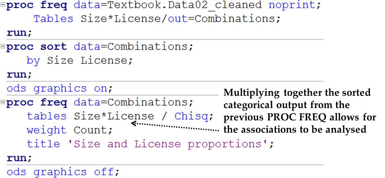
The following SAS code (given to you in the file “SASCode15c Two-way chi square test”)
will give a variety of the most basic categorical variable relational statistics for
the textbook example of associating Size and License:
Figure 15.8 Basic SAS Code for Associating Categorical Variables
This will first produce a table like that seen in Figure 15.9 Initial table of statistics for categorical variable associations below:
Figure 15.9 Initial table of statistics for categorical variable associations

The following sections will discuss these and other statistical tests for associating
multiple categorical variables.
Testing General Association between Categorical Variables
Similar to the one-variable example, you can test generally for association between
categorical variables, even if you have no sense of exactly how the association happens,
no assumption of dependence where one variable is causing the other, and so on.
Here, instead of a benchmark set of probabilities, the variables are compared directly
to each other. There are two sets of tests:
-
In Figure 15.9 Initial table of statistics for categorical variable associations above, the “Chi-Square” and “Likelihood Ratio Chi-Square” fulfill the test for general association of categorical variables. As before, a significant (low) p-value suggests that the categorical variables are related, as seen in Figure 15.9 Initial table of statistics for categorical variable associations, where the p-values of < .001 suggest Size and License are associated.
-
Also useful are the final three tests in Figure 15.9 Initial table of statistics for categorical variable associations. The “Phi coefficient”, “Contingency Coefficient” and “Cramer’s V” statistic can be read in a similar way to correlation coefficients when the contingency table is a 2x2 format, where both variables have only two categories. (In a 2x2 table, the values run from -1 to +1, with larger absolute values indicating stronger associations.) In this case, size has three categories. In non-2x2 cases, the interpretations change somewhat. The Cramer’s V is probably the easiest to understand in this case: its boundaries change to run from 0 to 1 like an R² value in regression. Practically, so long as the number of rows and columns are not too different, you can still read these three scores like correlations. We see in Figure 15.9 Initial table of statistics for categorical variable associations that the Phi coefficient, Contingency Coefficient and Cramer’s V are all in the .30-.32 range, suggesting a moderate association between Size and License.
Testing Trend in Ordinal Variables
Because ordinal variables have a natural low-to-high order, combining them allows
for analyses of trend and inferences of dependency. In other words, you can get closer
to a regression-type idea, where you can test whether one ordinal variable tends to
have higher scores when another ordinal variable has lower or higher scores.
Note that binomial or dichotomous variables (those with only two values) can sometimes
be seen as ordinal. For example, in the textbook example we might possibly see License
as ordinal, because Freeware and Premium can be seen as progressive states of purchasing.
There are many possibilities for analyzing trend in ordinal data in SAS PROC FREQ.
In Figure 15.9 Initial table of statistics for categorical variable associations we see one such example, the Mantel-Haenszel Chi-Square test. This statistic can
test trend between two ordinal variables, or one ordinal variable and one two-category
binomial variable (Cody & Smith, 1997). If we were to stretch it to our discussion,
Size is ordinal and has three categories, and License has two categories and might
possibly be seen as ordinal. The p = .0641 suggests that License choice may depend
on Size of the customer at about a 94% confidence level. Examining the actual distribution
of cells in Figure 15.2 Crosstab example of relating two categorical variables does, however, suggest that linearity is not perfect (we see there that medium firms
indeed have a far higher incidence of Premium customers than Small firms, but that
the trend reverses somewhat for Big firms).
In addition, there are many other options in SAS to examine linearity in ordinal variable
combinations:
-
In the PROC FREQ SAS code in Figure 15.8 Basic SAS Code for Associating Categorical Variables, the “CMH” keyword requests the “Cochran-Mantel-Haenszel Statistics” which also test for dependency and trend.
-
Adding the keyword “Measures” gives many additional measures, including more versions of correlation coefficients and other powerful tests for trend.
-
Even more complex options exist in SAS, such as the powerful PROC CATMOD routine, which I do not cover in this introductory textbook.
This introductory book does not go further into the great many available tests and
measures in this area; the interested reader should access the SAS helpfiles (the
SAS/STAT 13.2 User’s Guide or the like) and other specific texts on this topic.
Further Testing Possibilities in Categorical Variable Association
There are many other types of tests that can be achieved when you associate categorical
variables. For instance:
Homogeneity of odds ratios tests: If you have more than two categorical variables associating at the same time, then
obviously the analysis becomes more complex. Typically, a core two-way analysis is
split by other variables. For instance, in the textbook example Size x License forms
the core categorical association. Now, say we add a third categorical variable regarding
customers, such as stock exchange Listed versus Unlisted. Now, SAS would create two
Size x License contingency tables, one for listed customers and one for unlisted.
Each could be examined separately, but what if you wish to assess the similarities
or differences between these two listed and unlisted tables? As illustrated in Figure 15.10 Homogeneity test for differences in contingency tables below, there are tests (e.g. the “Homogeneity of the Odds Ratios” test) that explicitly
test whether these split contingency tables are roughly similar or very different.
Figure 15.10 Homogeneity test for differences in contingency tables

Agreement tests: Contingency tables can be used to test the extent to which different raters assess
the same objects. For instance, two influential automotive journalists may each rate
a set of cars on an ordinal scale “Great,” “Good,” “Average,” “Below average,” or
“Terrible.” You could test the extent to which they agree by arranging their ratings
into a two-way table. Similar tests to those discussed above would apply.
Categorical measurements over time: If categorical measures are made at several periods in time, tests can be made to
see whether or not the responses differ over time.
Noninferiority and superiority tests: There are specific tests to compare certain categories. A classic application of
these tests is in pharmaceutical testing. To get a new drug to market, one of the
tests you will typically do is to show statistically that its outcomes are not significantly
worse than some benchmark – perhaps the benchmark provided by other drugs already
on the market. This is a noninferiority test. Say that you are examining drug side effects of a new cholesterol medication.
You might set out to show that your drug does not have significantly worse side effects
than other competitor drugs. Your contingency table would compare drug types (one
categorical variable) against numbers of reported side effects (the second categorical
variable). Superiority, on the other hand, seeks to show clear advantages of your category over others.
You may seek to show that your cholesterol drug has statistically significantly fewer
side effects than your competitors. Contingency table tests exist for each of these
situations.
As noted in the previous section, there are many SAS procedures other than PROC FREQ
which specialize in associations of categorical data. Perhaps foremost among these
is PROC CATMOD, which allows for advanced modeling of these situations, and which
should be the next stop for many readers interested in this area once the essential
skills mentioned here have been conquered.
Last updated: April 18, 2017
..................Content has been hidden....................
You can't read the all page of ebook, please click here login for view all page.