In Chapter 3 we discussed the concept of variable spread. Apart from statistics like the mean that represent the centrality of the data in a variable, we also need statistics that speak to the extent to which the data spreads away from the middle. The following are some common statistics that measure spread.

A standard deviation (SD) is a score that we can use for the spread of data away from an average, although only in the case of continuous (interval or ratio) data. There is also a related measure called a variance. Take a look at Figure 7.1 Example of a final descriptive statistics table on page 68 which gives standard deviations of some variables.

The standard deviation and variance are very important, forming the basis for a great proportion of the world of statistics. Therefore, understanding the concept is important.

The standard deviation gives a measure of the average dispersion of a variable around the average. Precisely, if the variable is normally distributed in the complete population, the standard deviation tells us the distance away from the mean within which approximately 66% (two-thirds) of the population would be expected to lie.

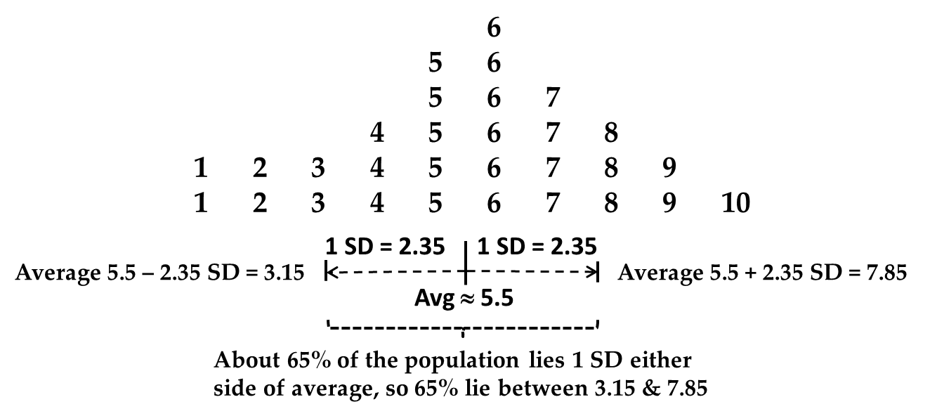
For an example, let us analyze some new performance appraisal data as seen in Figure 7.5 Pictorial representation of standard deviation . The data in Figure 7.5 Pictorial representation of standard deviation has an average of 5.5 and a standard deviation of 2.35. This means that:

The crucial thing to remember about a standard deviation is that it captures a range of data within which most of the population (two-thirds) is expected to lie. Therefore, it reflects the representative spread of the data away from the mean.

The variance of a variable is the standard deviation squared. As stated, you need to understand this without necessarily having to know how it is calculated. The important thing is to remember that, like the standard deviation, the variance is a measure of variable spread.

Further reading on the meaning and use of the SD and variance can be done in any introductory statistics text.

The interquartile range (IQR) captures the data points representing the 25th highest ranked observation in the range to the 75th highest ranked observation. In other words, it represents the data points between which the middle 50% of the data lies.

Put differently, if you line up all the data points from the lowest to highest, the computer figures out which point has 25% of lowest points lying below it and which data point has the 25% biggest scores above it. The interquartile range is the distance between these two. See the “IQR” column in Figure 7.1 Example of a final descriptive statistics table for an example of this statistic.

As with the median (which is the 50th percentile), the IQR can be used for ordinal data, whereas the standard deviation should probably not. Also, you can also look at the IQR for continuous data.

There are some overall measures of spread for categorical variables, but the basic comparison of frequencies between categories is your basic approach. See the Frequencies of firm sizes in Figure 7.4 Example of frequency analysis of categorical data in SAS for an example.

Calculating the spreads of variables in SAS is done through the descriptive statistics modules in the same way as the mean and median. See Getting Descriptive Statistics in SAS for how to run these. To run the analysis, again:

If you want to do a good job of reporting your findings, report statistics in well formatted tables like that of Figure 7.1 Example of a final descriptive statistics table; don’t just copy the SAS tables directly into a report.