
The Aspects of Inaccuracy
The Two Faces of Inaccuracy
As we have discovered, when we do a
study we get a representative point-estimate statistic. The real question
behind accuracy is how confident we can be that this statistic represents
the true, actual population statistic (assuming the sample is a good
representation of the population).
Therefore, accuracy
is all about how well our sample statistic reflects the true population
statistic. Imagine that you could know the true population value (you
cannot of course, but imagine this). Simplistically, the true population
statistic might be characterized as existing or not existing in reality.
The question is whether your statistical test can adequately reflect
what exists in reality.
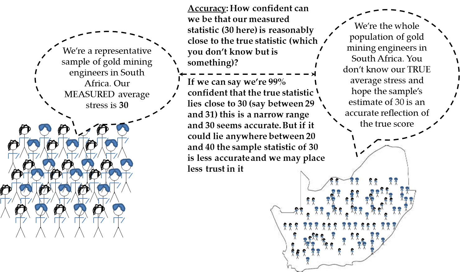
This principle is reflected
in Figure 12.5 Illustration of accuracy issue in which a
sample of South African mining engineers is tested for stress levels,
with a score of 30 on some stress scale (say out of 100).
The question for the
researcher is how much confidence we can put in this stress score.
If we conclude that we have a high level of confidence in the score
of 30 – say that at 95% confidence that the score lies between
29 and 31 (which is close to 30), then we can probably accept the
sample statistic as being accurate. On the other hand if we have the
statistic of 30 but it could lie anywhere between 20 and 40 then we’re
less sure of how representative of the truth the score is.
Figure 12.5 Illustration of accuracy issue
This thinking is even
more poignant when placed in the context of hypothesis testing, i.e.
when you seek to reject or accept certain hypotheses. Let us use an
example. In the chapter case example, imagine that you are a pharmaceutical
company testing a drug. Drug trials are very expensive, capable of
making massive revenue if they get approved, and can make a big difference
in peoples’ lives if they work (see the introductory case to
Chapter 18 for more on this issue). However, drugs can also be dangerous
or misleading if patients think that they work when they do not. Your
company could lose massive investments in marketing, get sued, or
lose reputation if you put a drug on the market that you claim works
but does not work in reality. The stakes are large and accuracy of
your drug trials is important. You have a hypothesis that you need
to test, namely, in this case we usually seek to reject the hypothesis
that the drug does not work and accept the alternative hypothesis
that the drug does work. These are stark, black-and-white decisions
that have huge consequences.
The hypothesis testing
scenario is helpful for thinking around the fact that accuracy is
actually a multidimensional concept, not just one thing. For this
discussion, look at Figure 12.6 Pictorial illustration of significance/power problems and Figure 12.7 Medical drug testing illustration of significance and power issues, which give
the two possible population truths (there is or is not a true effect,
i.e. the drug does or does not work in reality) and the possible sample
statistic testing outcomes (the tests find or do not find an effect,
i.e. we find the drug to work or to not work in the sample).
Figure 12.6 Pictorial illustration of significance/power problems

Obviously, in the drug
testing example, there are two scenarios you want to happen in any
given trial, namely:
-
The effect exists in reality and your test indeed finds a significant effect (top left cell). This cell is a good outcome: your statistical test reflects reality and your responses will be appropriate (accept that a finding exists). In the drug trial example, the drug does work in reality, your test confirms this, and your company can feel confident about marketing the drug.
-
The effect does not exist in reality and your test indeed finds a non-significant effect (bottom right). This cell is also a good outcome: your statistical test reflects reality and your responses will be appropriate (reject that a finding exists). In the drug trial example in Figure 12.7 Medical drug testing illustration of significance and power issues, your test shows little effect which reflects the truth that the drug does not work, and you can abandon the drug trial early and move on to more promising opportunities.
Figure 12.7 Medical drug testing illustration of significance and power
issues

However, there are two
cells left over in Figure 12.6 Pictorial illustration of significance/power problems and Figure 12.7 Medical drug testing illustration of significance and power issues that are bad
outcomes as follows:
-
Problem cell # 1 (the significance problem, a false positive). The effect does not exist in reality but your test finds a significant effect (top right). This is bad, because you now may assume that the effect exists but it does not, and your responses may be inappropriate. We call this a ”false positive,” because your test thinks there is an effect but this is false. We wish to minimize this risk. In the drug example of Figure 12.7 Medical drug testing illustration of significance and power issues, we think the drug works but it does not in reality. We start marketing it, and we mislead people, but we are probably eventually proved wrong and forced to withdraw the drug. We call this the significance problem, in most statistics texts it is the “Type I problem.” We often denote it as “alpha” or “α” which is the percentage/proportion chance of a false positive.
-
Problem cell # 2 (the power problem, a false negative). The effect does exist in reality but your test cannot find it (bottom left). This is bad, because you assume that the effect is absent but there is an effect in reality; again, your responses may be inappropriate. In many statistical texts, this is called the “Type II problem.” We obviously also wish to minimize this risk. In the drug example of Figure 12.7 Medical drug testing illustration of significance and power issues, we do not think the drug works but it does work in reality. We may abandon the drug trials, missing out on what should have been an opportunity to help people and make substantial profits. We call this the power problem.
In the following sections
I expand on these issues – the significance and power problems
– as well as the notion of hypothesis testing.
Accuracy Problem #1: Statistical Significance
More on Statistical Significance
As discussed above, statistical significance refers to
the chance of your statistic seeming to find a certain effect that
is wrong, i.e. not sufficiently representative of the true population
value. Another way to see significance tests is that they are formal
tests that some statistic that you have measured is sufficiently accurate
to be found again if you were to repeat your study, based on certain
assumptions and your sample. The more likely it is that our sample
statistic (say, the average stress of 30 of the sample in Figure 12.5 Illustration of accuracy issue) will be found
again in future studies, the more likely it is that it is the true
representation of the population.
The question of course
is how to measure significance practically. This is covered in the
rest of this section. Broadly, there are two different ways to measure
and therefore to assess the significance of a statistic. Before looking
at these, it is necessary to discuss the idea of confidence.
In statistics, “confidence”
is a concept about the probabilities of certain things happening.
We like to have high confidence in our findings (say 95% confidence)
because it means that less than 5% of the time we discover some statistical
finding that is actually wrong (i.e. the chance of being in the top
right quadrant of Figure 12.6 Pictorial illustration of significance/power problems).
Putting this another way, if I tell you I have found a statistical
estimate and have 97% confidence in it, this means that only 3% of
the time will I find a very different estimate of the same statistic
under the same condition: I can be confident in its accuracy.
Also important to understand
is that there are two uses for statistical significance tests, as
discussed next.
Two Uses of Statistical Significance Tests
Remember that statistical significance is all about accuracy:
how often will my statistic found in the sample be very different
from the same statistic if I do a similar study again?
There are two uses for
an estimate of the accuracy of a statistic:
Accuracy
Is Important For Its Own Sake
Have another look at
the gold mining example in Figure 12.5 Illustration of accuracy issue.
Here we have a sample of gold mining engineers and a statistic drawn
from that sample of Average Stress = 30. We then say that, instead
of focusing on the single estimate, we are 95% confident that this
average statistic lies somewhere between 29 and 31. Compare that with
95% confidence that the statistic is between 20 and 40. Obviously
the former range (where the lower and upper ends are only 1 away from
the average) makes us more confident about the single average of 30
than the latter (which stretches 10 points below and above the average).
Ultimately the really
experienced analyst, who is in tune with his or her data, will be
able to look at the accuracy of a given statistic and decide whether
the feasible range of the statistic indicates relative accuracy or
inaccuracy.
Having said this, there
is, in fact, a second very important use for accuracy statistics:
hypothesis testing.
Hypothesis
Testing
Often we wish to assess
a given statistic against a benchmark to see if is either close to
or far away from the benchmark. This is called hypothesis testing.
By far the most common type of hypothesis test is against the benchmark
of zero. Here, we have what is called the null hypothesis:
Null
hypothesis: “My statistic = 0”
For instance, a null
hypothesis might be “Increased sales due
to the promotion = 0”.
We often look to reject
the null hypothesis in favor of an “Alternative Hypothesis”
that the statistic is not zero, or specifically above or below zero,
so for instance:
Alternative
Hypothesis: “Increased sales are not 0” or “Increased
sales > 0”
For instance, in the
pharmaceutical trial we might have the null hypothesis that the drug
has no effect on the symptoms. Say our average effect found in the
trial is a reduction in arthritis swelling by 12%. This is obviously
not equal to zero, but how confident are we about the fact that it
is in fact not too close to zero to tell the difference, remembering
that this statistical number has a range? Our research question might
say that takers of the drug experience improvement significantly higher
than zero. So the null hypothesis is “Improvement
from the drug = 0” and the alternative
hypothesis is “Improvement from the drug
> 0”.
Hypothesis testing is
the basis for most scientific and industrial testing involving statistics.
As discussed later, it is a very dangerous thing, however, when misunderstood,
largely because showing that a statistic is probably not zero does
not mean that it is also big or important in size. As reinforced in
this chapter, size or magnitude of the statistic is the real issue
of importance. Accuracy – which helps in hypothesis testing
– is an important consideration but size is foremost. I will
discuss this problem later in the text.
Now, understanding confidence
and the uses of statistical significance tests, we are ready to start
looking at two measures of statistical significance that use the concept.
The two most common significance measures are confidence intervals
and p-values, as discussed in the next two sections.
Significance Method # 1: Confidence Intervals
When we generate a single point value
statistical estimate such as an average, this has the huge down-side
of not reflecting anything about accuracy. Ultimately, it is far more
useful if we can say something like “with a certain amount
of confidence, the value of this statistic lies between X and Y,”
or using a more specific example “with 95% confidence this
average lies between 1,104 and 2,345.” This is a confidence
interval.
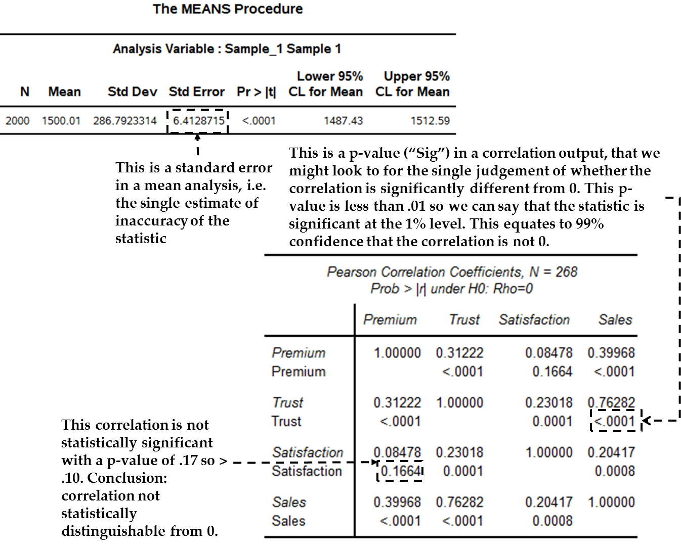
Confidence intervals
are possibly the most powerful and useful way of measuring and assessing
statistical significance, and in fact a statistic generally. Figure 12.8 SAS example of statistics assessing accuracy of a mean shows a specific
statistical output for the mean on our consumption data, including
a 95% confidence interval[1] .
In the figure you can see that the point estimate of the mean is 1500.01
and the 95% confidence interval is between 1487.70 and 1512.91.
Figure 12.8 SAS example of statistics assessing accuracy of a mean

You can generate confidence
intervals at various levels other than 95% (such as 99%) in most statistical
packages. Why are confidence intervals so useful?
-
First, confidence intervals give a more realistic picture of your statistic, providing direct assessments of accuracy in the measurement of the statistic. For example, in Figure 12.8 SAS example of statistics assessing accuracy of a mean the 95% confidence interval is the range R1487.43 - R1512.59. The analyst is able to interpret this range directly as a judgment of relative accuracy.
-
Second, confidence intervals are used to test specific hypotheses about the statistic, as discussed earlier. For example, say we had wanted to test whether average spending was significantly higher than a return-on-investment break-even figure of $1,250. In Figure 12.8 SAS example of statistics assessing accuracy of a mean the fact that this entire range of values in the confidence interval ($1487.43 to $1512.59) is higher than $1,250 tells us that, with 95% confidence, average spending in this sample is greater than the $1,250 break-even. As stated earlier, more often the hypothesis is that the interval does not contain zero – in which case you are saying “I bet that this statistic is significantly bigger or smaller than zero.” However, confidence intervals have the added advantage that they can test against any benchmark, not just zero.
Significance Method # 2: Single Inaccuracy Estimates & P-Values
Also available for most statistics
are single values that in some way reflect relative inaccuracy. For
instance, many statistics come with another value called the standard
error, which reflects how inaccurate that statistic is (i.e. how well
the statistic represents the population). The bigger the standard
error or other inaccuracy number, the less accurate we think the statistic
is. In Figure 12.8 SAS example of statistics assessing accuracy of a mean we see a column
called “Std. Error” which gives the measure of relative
inaccuracy for the average spending figure of R1,500.
To actually assess a
raw measure of inaccuracy, like the standard error, can be difficult
or close to impossible. As a result, we usually translate this inaccuracy
number into a standard value called a p-value (“probability
value”).
Most important to know
is that p-values always test the null hypothesis as discussed above,
where the null hypothesis is that the statistic is zero. Unlike confidence
intervals, which can assess accuracy for its own sake or can test
benchmarks other than zero, p-values always refer to the “Statistic
= 0” null hypothesis.
As an illustration of
p-values, let’s continue with the drug testing scenario. Say
that you wish to test an HIV/AIDS drug. You give one group of HIV
patients the drug, and compare their reactions to a control group
that is not given the drug. Most importantly, you wish to compare
a blood statistic called the “CD4 count” between the
groups. If your drug works then you expect to see a better change
over time in CD4 counts for the group that gets the drug than for
the group that does not. Therefore, your null hypothesis (which you
hope to reject) is:
Hull
hypothesis: The drug makes no difference in CD4 counts between the
two groups (or, more formally, the difference between the two groups
= 0).
The alternate hypothesis
(for which you hope to find evidence) is:
Alternate
hypothesis: The drug leads to better CD4 counts in the group given
the drug (or, more formally, CD4 for the group given drug –
CD4 for the group not given drug > 0).
Where does the p-value
come into all this? Well, say that your trial comes up with the conclusion
that changes in CD4 counts are on average 10 points better in the
group given the drug. Assuming you have designed the drug trial to
screen out all other possible causes, there are two remaining possible
reasons for this difference, namely a) the drug caused the difference,
and b) the drug caused little difference and really the differences
are just due to sheer random chance (people react randomly to things
all the time).
Which is it? If the
difference in CD4 is completely random and not due to the drug then,
even though there is some numerical difference, actually the null
hypothesis (difference = 0) is true. If the difference is big and
accurate enough to rule out the null hypothesis (difference > 0)
with a certain level of confidence, then we have evidence to suggest
that the drug makes a difference.
The p-value is used
for such hypothesis-based decisions. The p-value essentially tells
you how likely it is that the null hypothesis is true compared to
your found statistic, or that your statistic is due to random chance.
Say I tell you that given the CD4 differences between the two groups
and the inaccuracies, there is a 3% chance that the difference is
actually just zero. In other words that although you found a difference
of 10, this is just a result of random reactions and the difference
could just as easily be zero, at the same level of confidence. The
3% is the p-value, and you may essentially say “I’m
happy with the 3% chance of randomness. On the flip side this means
that I can be 97% confident that my drug trial result is sufficiently
far away from zero and accurate to be bigger than zero!”
This is then the primary
use of the p-value: to provide an assessment of your statistic versus
random chance. The lower the p-value, the greater the chance that
your statistic is not random chance.
Figure 12.9 Hypothesis testing and p-values in the drug trial example: The problem below provides
a courtroom metaphor of the basic hypothesis test issues, using drug
testing as an example.
Figure 12.9 Hypothesis testing and p-values in the drug trial example:
The problem

Figure 12.10 Hypothesis testing and p-values in the drug trial example: The scientific
test below illustrates
the p-value hypothesis testing response to such research questions.
Figure 12.10 Hypothesis testing and p-values in the drug trial example:
The scientific test

Therefore, the p-value
is a direct assessment of the probability of finding a statistic when
this is wrong in the population, i.e. a false positive, or “alpha”
(α) as shown in the top
right quadrants of Figure 12.6 Pictorial illustration of significance/power problems.
If we are not using
confidence intervals, p-values are what we usually use in order to
assess relative accuracy of a statistic. Appendix A of this chapter
explains how we get from the measure of inaccuracy to the p-value,
but you don’t really need to know this. The basic analyst can
bypass the measure of inaccuracy and look directly at the p-value.
The rest of this section therefore explains the use of p-values.
The following bullets
summarize the use of p-values:
-
P-values are expressed in proportions that equate to the opposite of confidence relative to some benchmark, essentially measuring lack of confidence. For example, we may obtain a p-value of 0.02. In simple terms, this would equate to 2% ”lack of confidence” in our result; therefore we would be able to say that we have 98% statistical confidence in our result rather than the benchmark.
-
Therefore, the smaller the p-value the more accurate our statistic. We usually say that if the p-value is less than .05 or .01 then the statistic is significant at the 5% or 1% level, which equates to 95% and 99% confidence respectively.
-
A p-value of 5% or 1% means that there is a 5% or 1% chance of wrongly rejecting the hypothesis that the estimate is not accurate. When you do research and measure a statistic, you are implicitly proposing that your statistic is accurate. The standard error provides a measure of how variable and therefore potentially inaccurate your statistic might be. If our statistic is so variable that we are not likely to find the same estimate again, then we would reject our research proposition that it is accurate. Based on this, we can conclude whether our statistic is sufficiently accurate.
-
Normally we want a low p-value (less than, say, 0.05), because this reflects the conclusion that, in less than (say) 5% of similar studies, we would expect to find a significantly different statistical estimate to the one that we found.
Figure 12.11 Interpretation of p-values summarizes
the interpretation of p-values.
Figure 12.11 Interpretation of p-values

P-values
with SAS as an Example
In SAS, p-values are
designated “Pr >.” Figure 12.12 Mean and correlations illustrating standard error and p-values shows two outputs.
On the top is the earlier statistical output for our mean, and highlights
the standard error. We would typically not try to interpret this directly.
Instead, we would usually look to a p-value. The lower picture shows
the p-values for some correlations (see the “Pr < |r|”
rows) – the lower the p-value the more accurate our statistic;
here the p-value is less than .0001 so we believe it is very accurate,
as discussed in the figure.
Figure 12.12 Mean and correlations illustrating standard error and p-values
Therefore, if you are
not using confidence intervals (or if you supplement the use of intervals
with p-values), look for the p-value to be lower than .05 or .01 and
interpret accordingly. (Note that some fields of study allow for higher
p-values, such as .10 equating to significance at 10% and therefore
90% confidence).
Bootstrapping as a Better Way of Assessing Significance
There is a technique called bootstrapping (Efron
& Tibshirani, 1993), which is usually a superior method for generating
confidence intervals for statistics. This is an alternative to the
usual way of generating confidence intervals (I explain the usual
basic method in Appendix A).
Bootstrapping is often
better because it usually produces more accurate confidence intervals.
Many statistical packages make it possible for you to bootstrap your
statistics at the click of a button. SAS has powerful abilities to
bootstrap, but it is not an automated procedure (On the SAS website,
there is an easy-to-follow macro to achieve it for any SAS procedure.)
When you bootstrap,
you will generally find a section in the output that gives bootstrapped
confidence intervals for your statistic (see Figure 12.13 Output with both original and bootstrapped confidence intervals for an example),
and you can use and report these as the estimates of accuracy instead
of the usual confidence intervals.
Figure 12.13 Output with both original and bootstrapped confidence intervals

If you are interested
in the details, Appendix A briefly discusses how bootstrapping works,
and why it produces better confidence intervals. You do not necessarily
need to know all these details – if a statistical system makes
it available, you usually can use the technique.
There are some relatively
rare times you cannot bootstrap[2] , or where you must adjust
it before it will work. If you are doing an unusual statistical analysis
perhaps read up specifically on your type of analysis and bootstrapping.
One thing to note about
bootstrapping is that it often gives you slightly
different confidence interval limits every time you do it.
This is part of the process and to be expected.
Accuracy Problem #2: Statistical Power
Introducing Power
The
previous section assessed the statistical significance “Type
I” problem seen in the top right quadrant of Figure 12.6 Pictorial illustration of significance/power problems, i.e. the issue
that you might find an effect in your sample statistic that actually
does not line up with the population (a false positive). However,
there was another problem seen in the bottom left quadrant of Figure 12.6 Pictorial illustration of significance/power problems, namely the
chance of missing an effect that does exist in the population (a false
negative), otherwise known as the “power” or “Type
II” problem. You may recall the drug trial example (see Figure 12.7 Medical drug testing illustration of significance and power issues) in which statistical
significance may be the problem of finding that the drug works when
it doesn’t, and the power problem being not finding an effect
for the drug when in fact it does work. This section explains power
in more detail.
Understanding Power
Allow me to start explaining power by using an analogy
of a metal detector used to look for buried treasure. The power of
the metal detector dictates how easy it is for it to locate a treasure:
-
The more powerful the metal detector, the more likely it is that a deeply-buried treasure will be found.
-
A more obvious treasure (a bigger and less-deeply buried one) can also be picked up by a weaker detector.
-
If the metal detector is too weak to pick up the treasure, it will of course not locate it, which is highly undesirable.
-
An exceptionally strong metal detector might pick up every little bit of metal instead of only locating larger loads of metal.
The power of a statistical
test is like the power of the metal detector. It expresses the ability
or sensitivity of a statistical test to detect an effect. There exists
the unfortunate problem that you may not find statistical significance
for an effect that you should otherwise have found (your test is not
sensitive enough). Power also has another side, which is that some
tests find everything to be statistically significant no matter how
small (your test is almost too sensitive). I discuss both aspects
below.
The Measurement of Power
Before understanding its elements and uses, it’s
useful to understand the overall measurement of power. Power is measured
as a proportion between 0 and 1, where 0 means that the test will
not find an effect and the closer to 1 the power score gets, the greater
the chance of finding an effect that does exist.
Is there a cut-off for
”good” power? Many statisticians prefer power > .80,
i.e. at least an 80% chance of finding an effect that exists. This
is debatable and depends partly on your research needs.
Figure 12.14 A statistical table in SAS including power shows an example
of a power statistic from SAS. The power analysis is for a type of
statistic that formally tests whether an average is significantly
different from zero.
Figure 12.14 A statistical table in SAS including power
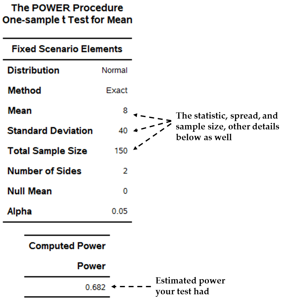
The data from Figure 12.14 A statistical table in SAS including power has the following
details:
-
The average of the variable = 8
-
The standard deviation of the variable = 40
-
The sample size = 150
The final statistic
assesses the power of the test. The power for this test is .68. Since
close to 1 is better, this is fairly low, indicting that if an effect
exists we may not have the ability to locate it (i.e. find it to be
statistically significant). I discuss more below what this may mean
and how to respond to it.
Having briefly discussed
statistical power and its basic measurement, the following sections
discusses two approaches to power as well as the elements of power.
The Elements of Power
Consider again the analogy of the metal detector. What
makes for the chance that you will find the buried treasure? The following
make it more likely you will find a treasure:
-
The amount of ground you cover with the metal detector looking for the treasure: Of the total ground available, the more ground that you cover, the more likely that you will find the treasure.
-
The size of the treasure: The bigger the size, the more likely that you will detect it.
-
How spread out the treasure is: If the treasure is spread out over much ground, it will be hard to detect. A closely condensed treasure will be easier to detect.
-
The chance you are willing to take of finding treasure that is not there: As you look for treasure you might also find other things like old, buried scrap metal. This wastes time and effort. Ironically, the more power, the more likely it is that you’ll find something small that you don’t want, a too-powerful metal detector will beep for anything from a paper-clip to a true treasure.
-
The type of treasure: Some metals may be easier to locate than others; smaller quantities of them will give off stronger signals.
Similarly, returning
to statistics, there exist various things that affect power of a statistical
test, as follows:
-
Sample size: The bigger your sample, the better the power of the test. This is because the bigger the sample, the more likely that your statistic will reflect the true population (up to the point at which your sample is perfectly large, i.e. it is the population, and then your sample statistic is the population statistic). Having more observations is like covering more ground in the treasure-hunt, it gives us a better chance of finding an effect that does exist. Obviously, though, bigger samples are harder and more expensive to get.
-
Effect size of the statistic: Just like a bigger treasure is easier to locate, a larger statistical point estimate will be easier to locate or confirm, therefore making overall power better. For instance, say you have a sample of size n = 100. With this sample size, a correlation of .15 is not significant at 5%, whereas a correlation of .20 is significant at 1%. The sample sizes are identical (n = 100); a major difference is the relative sizes of the two correlations.
-
The variability (variance or standard deviation) in the statistic: If the expected variability in the statistic is larger, then power is smaller, since there is less accuracy in the possible answers and a higher chance of not finding the correct value. The metal detector analogy here is a treasure that is more or less spread out – the same size treasure (say 100kg of gold) will have a stronger magnetic field and be easier to locate if it is clustered together (low spread) than if it is spread out (higher variance).
-
Your willingness to find an effect that isn’t there (the test α): Remember the significance problem (Type I error as denoted by α, equating to the p-value calculation) is the chance of a false positive (top right quadrant of Figure 12.6 Pictorial illustration of significance/power problems). When you do statistical testing, there is always a chance you might find a false positive. However, you might be willing to risk this to a greater or lesser extent. The test alpha is your willingness up-front to find effects that are not correct (false positives). Since power is the sensitivity of the test, higher power ironically also heightens the chance of a false positive. Therefore, the level of Type I error you are willing to accept affects the power of your test – the more you are willing to risk a false positive the more powerful your test will be to find a true effect. The treasure analogy here is your willingness to also find non-treasure metals. If you only want a 1% chance of thinking you’ve found treasure and digging up a car wheel, then whatever your metal detector you are less willing to dig up things that you find unless they are huge. This runs the risk that you’ll pass over a small but real treasure (a false negative risk, as seen in the bottom left of Figure 12.6 Pictorial illustration of significance/power problems). If you are willing to run a 10% chance of digging up false treasure instead, by implication your power with the same detector is higher because you will take more chances to dig, leading you both to more false positives but also more smaller treasures that you’d have passed over if you were more fussy.
-
The type of test: I also note that some statistical tests are inherently more powerful than others. As seen in the analogy of treasure that is more or less easy to find by nature, some statistical tests are simply more or less powerful. This has good and bad elements; remember that great power may mean everything looks significant, even the small stuff.
Power is therefore increased
when:
-
Sample sizes are bigger.
-
The raw statistical effect (point estimate of the statistic) is bigger.
-
The statistic is more accurate (less varied, usually proxied by how variable the data is).
-
Test alpha is higher (you are inherently more willing to accept Type I or false positive errors).
-
The test you are using is more powerful.
Typically, each of the
first four elements above is related to each other by an equation,
the form of the equation depending on which test is used. This text
won’t teach the equations, but they are quite easy to access.
Power Measured Before and After Testing
You can assess power before or after your study.
Assessing
Power Before a Study: “A Priori” Power Analysis
It is possible to analyze
aspects of power before even starting your research – we call
this a priori power analysis. Why would you want to do such a thing?
Usually, researchers want to know in advance of starting one of two
things: a) how big a sample they need to gather in order to achieve
their aim, or b) whether the sample they know they are going to get
will allow for sufficient power.
To assess how big a
sample you will need for a minimum level of power, you need the likely
values of the major elements of power as follows:
-
The minimum power level you are willing to settle for: As discussed, researchers often use minimum power of .80.
-
The raw statistical point-estimate desired: Say that in a drug trial you are able to provide a target level of improvement.
-
The variability (variance or standard deviation) of the effect: This is harder to access. However, figures for the population effect can be calculated or located based on similar studies elsewhere and the like.
-
The test alpha: As discussed earlier, you can decide on the level of Type I error you’re willing to accept. If you are willing to relax the alpha (allow a higher error) then your power issues are also relaxed. In the drug trial example you may decide that you do not need alpha of .05 equating to 95% confidence and a 5% chance of a false positive. Perhaps the drug has few side effects but if it works it will save lives: in this case, perhaps allowing for a higher (say 15%) chance of finding an effect but being wrong (and therefore marketing the drug) is deemed acceptable.
Using pre-guesses of each of these, equations
exist to estimate how big a sample your test will then need to achieve
the minimum power (Cohen, Cohen, West & Aiken, 2003). For an example,
see the SAS output in Figure 12.15 Measurement of a-priori power using SAS PROC POWER.
Figure 12.15 Measurement of a-priori power using SAS PROC POWER

If on the other hand
you know the sample size you will get, you can also turn such equations
around and calculate the power you will achieve. If you find the power
to be low, you can perhaps rethink aspects of your study such as the
sample, alpha, minimum effect size, etc.
Assessing
Power After a Study: “Post Hoc” Power Analysis
You can also assess
the power of a statistical estimate that has already been generated,
which we call ”post-hoc” analysis. Figure 12.14 A statistical table in SAS including power above shows
a post-hoc power analysis, which is the power the test has to assess
the ability of the test to find effects once the elements of the test
are known.
The problem with post-hoc
power analysis is that the test has already been computed, which means
that your options to deal with problems caused by power is now more
limited than when you figured out power in advance (a
priori). You do have options to respond reactively
to problems in power, so post-hoc analysis is useful too.
However, do not assume
you need to react to low post-hoc power. Low power is not always a
problem. If your statistical test finds an effect that has relatively
acceptable statistical significance despite relatively
low power, then power has not affected the situation. (True, had the
power been higher, the significance would have been put out of question.
However, significance is still OK here.) This situation of statistical
significance with relatively low power would happen only if there
was a very large effect with low variability or a very large sample.
Your response in this case would probably be to deal with the low
power, and especially to try to avoid low power in future replications
of your test.
The Two Main Power Problems
The following two power issues can arise.
The
Low Power Problem
If you have an effect
that seems worth taking into account but has poor significance (confidence
intervals that are too wide, high p-values, i.e. high chance of a
false positive) and it also has low power (say power < .80) then
you have a low power problem. For instance, you may have a statistic
with a p-value of .054 (with which you might not be satisfied) and
low power of .57. The issue is that normally we would want to conclude
that our effect is not statistically significant (at the 95% level)
but the simultaneously low power means that we cannot be sure of this.
Because we have low power, we lack the ability to find effects that
really exist. The poor significance could be a factor of the power
not necessarily of poor accuracy or effect size. Figure 12.16 Illustration of the low power problem illustrates
the low power problem graphically.
Figure 12.16 Illustration of the low power problem

Here we have a correlation
= .28, which may or may not be found to be statistically significant
depending on sample size. With low enough power, such a correlation
will be found to be non-significant (its confidence interval will
include zero). However, if the correlation of .28 is a correct representation
of the population correlation then improving power to find significance
is desirable. If the low power problem occurs (low power and non-significance),
then the guidelines discussed above apply to dictate your possible
remedies:
-
Increase the sample size: This will improve power but is expensive and hard to achieve. It also requires you to re-do all your statistical computations, since there will be new data. It is rarely the route taken.
-
Improve the variability of the statistic: As explained previously, the variability in the fundamental statistic affects power. You can sometimes improve variability by improving your model. Usually this improvement is achieved through better modeling of what data you do have, but better data collection in advance is best. For instance:
-
Reduce measurement error: You may have badly measured your core variables contributing to the effect and be able to revisit their measurement. For instance, if you used a multi-item scale, can you revisit the process you went through to get final scores, and improve it? Power may be improved if reliability of measurements is improved.
-
Include other variables: Aside from the variables you have already used, are there others you might add to the analysis to reflect the true context of your effect better? For example, in calculating a correlation between two variables it is possible to estimate a correlation which is simultaneously controlled, for the effect of other variables. This may improve power. We will see this sort of thinking in the regression and comparison of means chapters.
-
Improve the modeling of the original variables: Even when we have a statistic and no way to improve the data or add other variables, we may be able to improve the basic modeling technique used.
-
-
Increase your test alpha: Recall that your power is affected by your test alpha (your willingness to accept false positives, i.e. worse significance levels). You can alter the significance levels that you test for (the test alpha) when you test, which will improve power. The default of most statistical programs is to test at the alpha = .05 level. However, if (and only if) you conclude that your study context can accept a lower Type I error rate (e.g. alpha = .10), then you can retest at this level and power will improve. However, this approach will not affect your actual p-values, so actual Type I error still stays as is. The difference is that power will increase, because you don’t need as much to find an effect. Therefore, if your p-value was very poor (say p = .24) then this is not really a solution because allowing yourself to accept a 10% error is still no good if error is 24%.
The
High Power Problem
The other potential
problem is that of excessively strong power that leads even the smallest
effects to be statistically significant. This generally occurs when
sample sizes are very big. This is frankly not a problem so long as
the researcher does not put statistical significance ahead of size.
Just because a statistic is significant (p-value is low or a confidence
interval is narrow) does not mean that the statistic is important.
As discussed in the first sections of this chapter, a statistic is
important when its raw magnitude is big. We desire a big and accurate
statistic, but accuracy is secondary to size: tiny and accurate means
you have practically no effect, despite statistical significance.
For instance, in Figure 12.17 Illustration of the high power problem there
is a tiny correlation of .06 which is very close to zero. The figure
also shows this correlation to be statistically significant as its
confidence interval lies between .02 and .10. However, this significance
merely acts to confirm that the correlation is small; we would never
now say such a correlation is worth taking seriously. Therefore, when
you have strong power, statistical significance, and seemingly low
effect size, you have the problem of high power. In such a case you
should probably accept that your statistic may be statistically significantly
greater than zero but that this is a technicality and it is functionally
very small and not important.
Figure 12.17 Illustration of the high power problem

Last updated: April 18, 2017
..................Content has been hidden....................
You can't read the all page of ebook, please click here login for view all page.