Issue # 1: Size of a Statistic
Size Matters!
Also called
the magnitude, size represents
the literal numerical size, impact or importance of a statistic. For
example, if you have calculated an average, is it a big average in
its context? If you have calculated a correlation that represents
linear association, is it a big or small correlation and therefore
a strong or weak linear association? Figure 12.1 Example of statistical output for the mean or average of a variable shows an example
of an output calculating the mean of spending on a product by business
customers. The key number is the literal size of the average, so we
see that in our sample, customers spend about $1,500.01 (rounded to
$1,500) per month.
Figure 12.1 Example of statistical output for the mean or average of a
variable

Size
or magnitude is really the important attribute of a statistic.
The numerical size of a statistic will determine the impact that the
underlying construct realistically has on the world around it, and
therefore its importance. Never lose sight of the fact that size of
any statistic is the real issue at hand.
Interpreting the Size of a Statistic
Interpreting Raw Size
Once you have done an
analysis, you should always try to interpret the size of a statistic
in terms that represent its real meaningfulness.
This is usually only
possible when you have a frame of reference for your data, such as
a sense of the spread of the data or some comparison number for what
is ”big” or ”small.” For instance, a Sales
number of $1,500 is meaningless on its own. It takes on meaning only
when you as the analyst understand more information about the Sales
data in general. Historical Sales data could have such a spread and
average that $1,500 is big, small or normal in historical context.
However, direct interpretation
of statistics is often not easy or even possible. This can happen
for two main reasons:
-
The underlying data may be such that you do not necessarily know what is big or small.
-
Many statistics have no immediate connection to underlying data anyway – they are measurements of concepts about data or associations between variables, but measured in ways that most analysts could not interpret directly. I provide an example in the next main section on standardized statistics.
Despite the fact that
many statistics cannot easily be interpreted directly, always strive
to interpret the actual magnitude of your statistics.
There are two things
to consider when considering the raw size of your statistic, as explained
in the next two sections.
Looking at the Size of Your Statistic on Its Own
Hopefully your statistic
has its own meaning or interpretation that means something to you.
For instance, in our example of customers, the average spend of $1,500
per customer is possibly intrinsically meaningful. You may look at
changes in this value over time, compare it to your competitors, or
find other ways of assessing its meaning to you.
If you think about it,
you will realize that every statistic is meaningless without some
benchmark against which to compare it. In the previous example, comparison
was needed against historical levels, competitors, etc.
Extrapolating Your Statistics to Further Business Implications
This book focuses on business statistics,
therefore considering business implications of your findings –
such as financial or strategic implications – is highly desirable.
Even if you are reading this and you are not a business person, you
may wish to consider the business consequences of your research, perhaps
in monetary terms. Perhaps you are a medical or pharmaceutical researcher.
Converting your statistics to monetary terms may help you understand
the commercial feasibility and pricing of your drug or the impact
of your suggestions on the hospital’s pricing policy. If you
are in education you could comment on the impact on school fees, textbook
pricing, or the economy. In zoology you could consider the impact
of your findings on the entrance tickets for parks or zoos, or on
the number of park rangers required.
Also, the lessons taught
in this book can be extended to other end outcomes, not just money.
For instance, the medical world sometimes measures “Quality
of Life Years” (QUALYs) as a patient outcome. One could use
the same sort of procedure as for monetary extrapolation.
Chapter 17 discusses
extrapolation of statistics to financial outcomes in particular in
more detail.
Sometimes the raw size
of a statistic is hard to interpret. The next section discusses a
way around this.
Standardized Statistics
Sometimes the data you are using
is measured in hard-to-interpret ways. For example, you may ask twenty
questions in a survey all designed to assess stress, and each question
may be measured on a 1-5 scale. You may then combine all these stress
answers for each person into an overall stress index. What does this
index really mean though? You can tell if a person is more or less
stressed by their position on the scale, but if I tell you that average
stress is a score of 67, what does this really mean? If someone improves
from 67 to 62 how good is this really? Such a scale, measured as it
is in arbitrary units, is hard to interpret directly.
In other cases, statistical
analysis gives us some statistical estimate that, by its own nature,
is difficult to interpret directly.
In these cases, statistical
packages often give us standardized values for the size of a statistic.
Standardized (sometimes called normalized) statistics are very useful
in these cases, because they translate something that may be hard
to interpret into a standard scale with well-understood properties
and cut-offs.
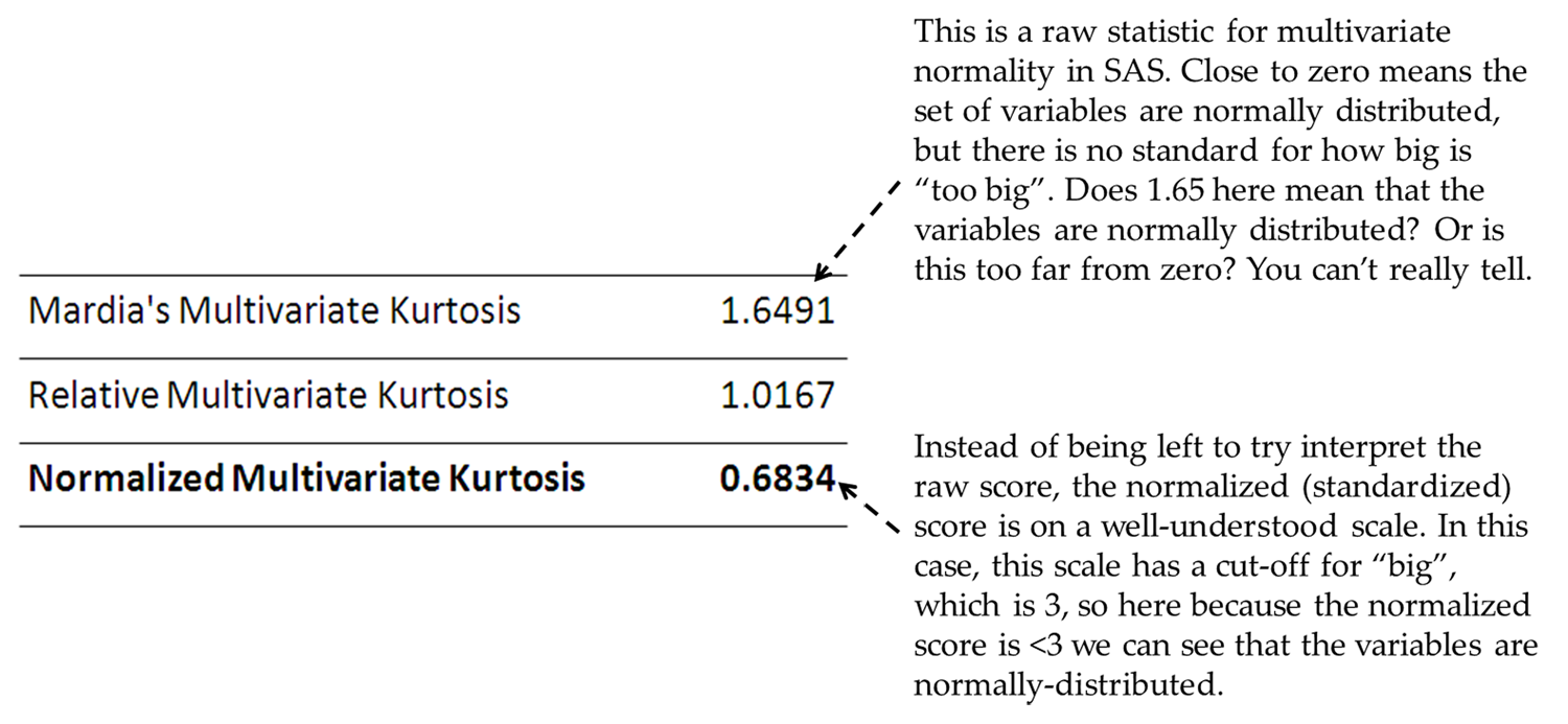
For instance, Figure 12.2 Example of a standardized (normalized) statistic shows an example
of a statistical output called the “Mardia measures of multivariate
kurtosis” (don’t worry about the terminology for now).
These measures assess the extent to which a set of variables are normally
distributed, not only individually but as a whole set.
As seen in Figure 12.2 Example of a standardized (normalized) statistic,
the raw statistic assessing the normality of the variables is called
the “Mardia Multivariate Kurtosis”. Technically, this
Mardia score needs to be zero for perfect normality. But it is not
– in the example the score is 1.65. The question is whether
this is too far from zero? What should we conclude: does our statistic
tell us that the variables are not normally distributed because 1.64
is not zero? Or is it close enough to zero to conclude that the variables
are normally distributed? Unfortunately we cannot really tell, because
the raw Mardia score has no recognizable cut-offs.
Figure 12.2 Example of a standardized (normalized) statistic

Instead, SAS provides
you with a ”Normalized Multivariate Kurtosis” score,
which is standardized onto a scale that does have a known cut-off.
On this particular standardized scale, anything bigger than 3 is usually
considered potentially big enough that it may be far from zero. Here
we see that the Normalized Multivariate Kurtosis score is only .68,
which is smaller than 3, so we would probably conclude that our variables
are normally distributed. It is the provision of an extra standardized
statistic that enabled us to make this conclusion, because the original
raw Mardia statistic was hard to interpret.
Note that this is only
one of many examples. Many other examples exist of standardizing statistics
so that the relative size can be ascertained. As you will see in the
next two chapters, certain more advanced measures of association between
variables come with standardized values so that they can be read as
though they are correlations, because we understand correlations well.
You should always try
to use raw, unstandardized values for statistics if you are able to
assess them in their units, because it is the raw values that reflect
the actual impact of the statistic, as discussed earlier under the
magnitude discussion. Standardized values are very useful as extra
analyses and especially useful if you cannot use the raw statistics.
Each time you use a standardized statistic, you need to look up the
particular rules for what a ”big”’ or ”small”’
standardized value is in the context of that statistic.
Last updated: April 18, 2017
..................Content has been hidden....................
You can't read the all page of ebook, please click here login for view all page.
