
4.5 Designing with Computing Platforms
In this section we concentrate on how to create a working embedded system based on a computing platform. We will first look at some example platforms and what they include. We will then consider how to choose a platform for an application and how to make effective use of the chosen platform.
4.5.1 Example Platforms
The design complexity of the hardware platform can vary greatly, from a totally off-the-shelf solution to a highly customized design. A platform may consist of anywhere from one to dozens of chips.
Open source platforms
Figure 4.21 shows a BeagleBoard [Bea11]. The BeagleBoard is the result of an open source project to develop a low-cost platform for embedded system projects. The processor is an ARM Cortex™-A8, which also comes with several built-in I/O devices. The board itself includes many connectors and support for a variety of I/O: flash memory, audio, video, etc. The support environment provides basic information about the board design such as schematics, a variety of software development environments, and many example projects built with the BeagleBoard.
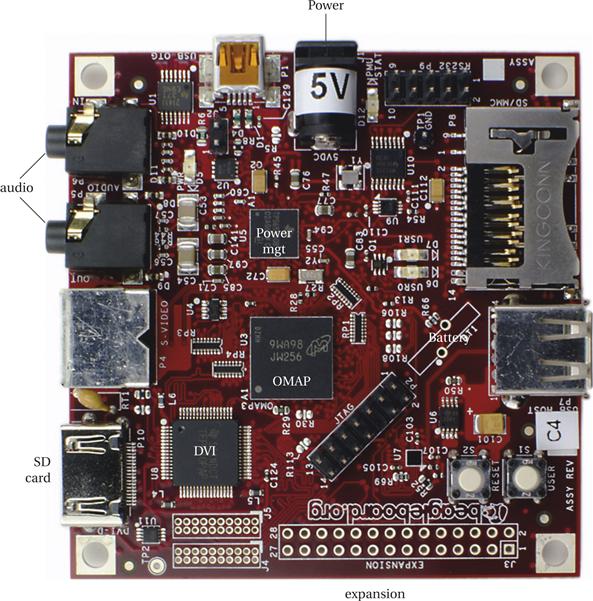
Figure 4.21 A BeagleBoard.
Evaluation boards
Chip vendors often provide their own evaluation boards or evaluation modules for their chips. The evaluation board may be a complete solution or provide what you need with only slight modifications. The hardware design (netlist, board layout, etc.) is typically available from the vendor; companies provide such information to make it easy for customers to use their microprocessors. If the evaluation board does not completely meet your needs, you can modify the design using the netlist and board layout without starting from scratch. Vendors generally do not charge royalties for the hardware board design.
Figure 4.22 shows an ARM evaluation module. Like the BeagleBoard, this evaluation module includes the basic platform chip and a variety of I/O devices. However, the main purpose of the BeagleBoard is as an end-use, low-cost board, while the evaluation module is primarily intended to support software development and serve as a starting point for a more refined product design. As a result, this evaluation module includes some features that would not appear in a final product such as the connections to the processor’s pins that surround the processor chip itself.
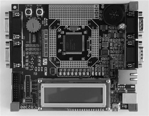
Figure 4.22 An ARM evaluation module.
4.5.2 Choosing a Platform
We probably will not design the platform for our embedded system from scratch. We may assemble hardware and software components from several sources; we may also acquire a complete hardware/software platform package. A number of factors will contribute to your decision to use a particular platform.
Hardware
The hardware architecture of the platform is the more obvious manifestation of the architecture because you can touch it and feel it. The various components may all play a factor in the suitability of the platform.
• CPU: An embedded computing system clearly contains a microprocessor. But which one? There are many different architectures, and even within an architecture we can select between models that vary in clock speed, bus data width, integrated peripherals, and so on. The choice of the CPU is one of the most important, but it cannot be made without considering the software that will execute on the machine.
• Bus: The choice of a bus is closely tied to that of a CPU, because the bus is an integral part of the microprocessor. But in applications that make intensive use of the bus due to I/O or other data traffic, the bus may be more of a limiting factor than the CPU. Attention must be paid to the required data bandwidths to be sure that the bus can handle the traffic.
• Memory: Once again, the question is not whether the system will have memory but the characteristics of that memory. The most obvious characteristic is total size, which depends on both the required data volume and the size of the program instructions. The ratio of ROM to RAM and selection of DRAM versus SRAM can have a significant influence on the cost of the system. The speed of the memory will play a large part in determining system performance.
• Input and output devices: If we use a platform built out of many low-level components on a printed circuit board, we may have a great deal of freedom in the I/O devices connected to the system. Platforms based on highly integrated chips only come with certain combinations of I/O devices. The combination of I/O devices available may be a prime factor in platform selection. We may need to choose a platform that includes some I/O devices we do not need in order to get the devices that we do need.
Software
When we think about software components of the platform, we generally think about both the run-time components and the support components. Run-time components become part of the final system: the operating system, code libraries, and so on. Support components include the code development environment, debugging tools, and so on.
Run-time components are a critical part of the platform. An operating system is required to control the CPU and its multiple processes. A file system is used in many embedded systems to organize internal data and as an interface to other systems. Many complex libraries—digital filtering and FFT—provide highly optimized versions of complex functions.
Support components are critical to making use of complex hardware platforms. Without proper code development and operating systems, the hardware itself is useless. Tools may come directly from the hardware vendor, from third-party vendors, or from developer communities.
4.5.3 Intellectual Property
Intellectual property (IP) is something that we can own but not touch: software, netlists, and so on. Just as we need to acquire hardware components to build our system, we also need to acquire intellectual property to make that hardware useful. Here are some examples of the wide range of IP that we use in embedded system design:
• run-time software libraries;
• software development environments;
• schematics, netlists, and other hardware design information.
IP can come from many different sources. We may buy IP components from vendors. For example, we may buy a software library to perform certain complex functions and incorporate that code into our system. We may also obtain it from developer communities on-line.
Example 4.1 looks at the IP available for the BeagleBoard.
Example 4.1 BeagleBoard Intellectual Property
The BeagleBoard Web site (http://www.beagleboard.org) contains both hardware and software IP. Hardware IP includes:
• schematics for the printed circuit board;
• artwork files (known as Gerber files) for the printed circuit board;
Software IP includes:
4.5.4 Development Environments
Although we may use an evaluation board, much of the software development for an embedded system is done on a PC or workstation known as a host as illustrated in Figure 4.23. The hardware on which the code will finally run is known as the target. The host and target are frequently connected by a USB link, but a higher-speed link such as Ethernet can also be used.
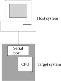
Figure 4.23 Connecting a host and target system.
The target must include a small amount of software to talk to the host system. That software will take up some memory, interrupt vectors, and so on, but it should generally leave the smallest possible footprint in the target to avoid interfering with the application software. The host should be able to do the following:
A cross-compiler is a compiler that runs on one type of machine but generates code for another. After compilation, the executable code is typically downloaded to the embedded system by USB. We also often make use of host-target debuggers, in which the basic hooks for debugging are provided by the target and a more sophisticated user interface is created by the host.
We often create a testbench program that can be built to help debug embedded code. The testbench generates inputs to stimulate a piece of code and compares the outputs against expected values, providing valuable early debugging help. The embedded code may need to be slightly modified to work with the testbench, but careful coding (such as using the #ifdef directive in C) can ensure that the changes can be undone easily and without introducing bugs.
4.5.5 Debugging Techniques
A good deal of software debugging can be done by compiling and executing the code on a PC or workstation. But at some point it inevitably becomes necessary to run code on the embedded hardware platform. Embedded systems are usually less friendly programming environments than PCs. Nonetheless, the resourceful designer has several options available for debugging the system.
The USB port found on most evaluation boards is one of the most important debugging tools. In fact, it is often a good idea to design a USB port into an embedded system even if it will not be used in the final product; USB can be used not only for development debugging but also for diagnosing problems in the field or field upgrades of software.
Another very important debugging tool is the breakpoint. The simplest form of a breakpoint is for the user to specify an address at which the program’s execution is to break. When the PC reaches that address, control is returned to the monitor program. From the monitor program, the user can examine and/or modify CPU registers, after which execution can be continued. Implementing breakpoints does not require using exceptions or external devices.
Programming Example 4.1 shows how to use instructions to create breakpoints.
Programming Example 4.1 Breakpoints
A breakpoint is a location in memory at which a program stops executing and returns to the debugging tool or monitor program. Implementing breakpoints is very simple—you simply replace the instruction at the breakpoint location with a subroutine call to the monitor. In the following code, to establish a breakpoint at location 0 × 40c in some ARM code, we’ve replaced the branch (B) instruction normally held at that location with a subroutine call (BL) to the breakpoint handling routine:
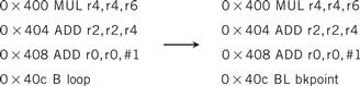
When the breakpoint handler is called, it saves all the registers and can then display the CPU state to the user and take commands.
To continue execution, the original instruction must be replaced in the program. If the breakpoint can be erased, the original instruction can simply be replaced and control returned to that instruction. This will normally require fixing the subroutine return address, which will point to the instruction after the breakpoint. If the breakpoint is to remain, then the original instruction can be replaced and a new temporary breakpoint placed at the next instruction (taking jumps into account, of course). When the temporary breakpoint is reached, the monitor puts back the original breakpoint, removes the temporary one, and resumes execution.
The Unix dbx debugger shows the program being debugged in source code form, but that capability is too complex to fit into most embedded systems. Very simple monitors will require you to specify the breakpoint as an absolute address, which requires you to know how the program was linked. A more sophisticated monitor will read the symbol table and allow you to use labels in the assembly code to specify locations.
LEDs as debugging devices
Never underestimate the importance of LEDs (light-emitting diodes) in debugging. As with serial ports, it is often a good idea to design in a few to indicate the system state even if they will not normally be seen in use. LEDs can be used to show error conditions, when the code enters certain routines, or to show idle time activity. LEDs can be entertaining as well—a simple flashing LED can provide a great sense of accomplishment when it first starts to work.
In-circuit emulation
When software tools are insufficient to debug the system, hardware aids can be deployed to give a clearer view of what is happening when the system is running. The microprocessor in-circuit emulator (ICE) is a specialized hardware tool that can help debug software in a working embedded system. At the heart of an in-circuit emulator is a special version of the microprocessor that allows its internal registers to be read out when it is stopped. The in-circuit emulator surrounds this specialized microprocessor with additional logic that allows the user to specify breakpoints and examine and modify the CPU state. The CPU provides as much debugging functionality as a debugger within a monitor program, but does not take up any memory. The main drawback to in-circuit emulation is that the machine is specific to a particular microprocessor, even down to the pinout. If you use several microprocessors, maintaining a fleet of in-circuit emulators to match can be very expensive.
Logic analyzers
The logic analyzer[Ald73] is the other major piece of instrumentation in the embedded system designer’s arsenal. Think of a logic analyzer as an array of inexpensive oscilloscopes—the analyzer can sample many different signals simultaneously (tens to hundreds) but can display only 0, 1, or changing values for each. All these logic analysis channels can be connected to the system to record the activity on many signals simultaneously. The logic analyzer records the values on the signals into an internal memory and then displays the results on a display once the memory is full or the run is aborted. The logic analyzer can capture thousands or even millions of samples of data on all of these channels, providing a much larger time window into the operation of the machine than is possible with a conventional oscilloscope.
A typical logic analyzer can acquire data in either of two modes that are typically called state and timing modes. To understand why two modes are useful and the difference between them, it is important to remember that an oscilloscope trades reduced resolution on the signals for the longer time window. The measurement resolution on each signal is reduced in both voltage and time dimensions. The reduced voltage resolution is accomplished by measuring logic values (0, 1, x) rather than analog voltages. The reduction in timing resolution is accomplished by sampling the signal, rather than capturing a continuous waveform as in an analog oscilloscope.
State and timing mode represent different ways of sampling the values. Timing mode uses an internal clock that is fast enough to take several samples per clock period in a typical system. State mode, on the other hand, uses the system’s own clock to control sampling, so it samples each signal only once per clock cycle. As a result, timing mode requires more memory to store a given number of system clock cycles. On the other hand, it provides greater resolution in the signal for detecting glitches. Timing mode is typically used for glitch-oriented debugging, while state mode is used for sequentially oriented problems.
The internal architecture of a logic analyzer is shown in Figure 4.24. The system’s data signals are sampled at a latch within the logic analyzer; the latch is controlled by either the system clock or the internal logic analyzer sampling clock, depending on whether the analyzer is being used in state or timing mode. Each sample is copied into a vector memory under the control of a state machine. The latch, timing circuitry, sample memory, and controller must be designed to run at high speed because several samples per system clock cycle may be required in timing mode. After the sampling is complete, an embedded microprocessor takes over to control the display of the data captured in the sample memory.
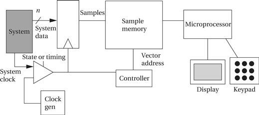
Figure 4.24 Architecture of a logic analyzer.
Logic analyzers typically provide a number of formats for viewing data. One format is a timing diagram format. Many logic analyzers allow not only customized displays, such as giving names to signals, but also more advanced display options. For example, an inverse assembler can be used to turn vector values into microprocessor instructions. The logic analyzer does not provide access to the internal state of the components, but it does give a very good view of the externally visible signals. That information can be used for both functional and timing debugging.
4.5.6 Debugging Challenges
Logical errors in software can be hard to track down, but errors in real-time code can create problems that are even harder to diagnose. Real-time programs are required to finish their work within a certain amount of time; if they run too long, they can create very unexpected behavior.
Example 4.2 demonstrates one of the problems that can arise.
Example 4.2 A Timing Error in Real-Time Code
Let’s consider a simple program that periodically takes an input from an analog/digital converter, does some computations on it, and then outputs the result to a digital/analog converter. To make it easier to compare input to output and see the results of the bug, we assume that the computation produces an output equal to the input, but that a bug causes the computation to run 50% longer than its given time interval. A sample input to the program over several sample periods looks like this:
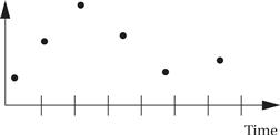
If the program ran fast enough to meet its deadline, the output would simply be a time-shifted copy of the input. But when the program runs over its allotted time, the output will become very different. Exactly what happens depends in part on the behavior of the A/D and D/A converters, so let’s make some assumptions. First, the A/D converter holds its current sample in a register until the next sample period, and the D/A converter changes its output whenever it receives a new sample. Next, a reasonable assumption about interrupt systems is that, when an interrupt is not satisfied and the device interrupts again, the device’s old value will disappear and be replaced by the new value. The basic situation that develops when the interrupt routine runs too long is something like this:
1. The A/D converter is prompted by the timer to generate a new value, saves it in the register, and requests an interrupt.
2. The interrupt handler runs too long from the last sample.
3. The A/D converter gets another sample at the next period.
4. The interrupt handler finishes its first request and then immediately responds to the second interrupt. It never sees the first sample and only gets the second one.
Thus, assuming that the interrupt handler takes 1.5 times longer than it should, here is how it would process the sample input:
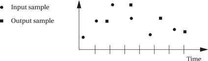
The output waveform is seriously distorted because the interrupt routine grabs the wrong samples and puts the results out at the wrong times.
The exact results of missing real-time deadlines depend on the detailed characteristics of the I/O devices and the nature of the timing violation. This makes debugging real-time problems especially difficult. Unfortunately, the best advice is that if a system exhibits truly unusual behavior, missed deadlines should be suspected. In-circuit emulators, logic analyzers, and even LEDs can be useful tools in checking the execution time of real-time code to determine whether it in fact meets its deadline.