
5.4 Assembly, Linking, and Loading
Assembly and linking are the last steps in the compilation process—they turn a list of instructions into an image of the program’s bits in memory. Loading actually puts the program in memory so that it can be executed. In this section, we survey the basic techniques required for assembly linking to help us understand the complete compilation and loading process.
Program generation work flow
Figure 5.10 highlights the role of assemblers and linkers in the compilation process. This process is often hidden from us by compilation commands that do everything required to generate an executable program. As the figure shows, most compilers do not directly generate machine code, but instead create the instruction-level program in the form of human-readable assembly language. Generating assembly language rather than binary instructions frees the compiler writer from details extraneous to the compilation process, which includes the instruction format as well as the exact addresses of instructions and data. The assembler’s job is to translate symbolic assembly language statements into bit-level representations of instructions known as object code. The assembler takes care of instruction formats and does part of the job of translating labels into addresses. However, because the program may be built from many files, the final steps in determining the addresses of instructions and data are performed by the linker, which produces an executable binary file. That file may not necessarily be located in the CPU’s memory, however, unless the linker happens to create the executable directly in RAM. The program that brings the program into memory for execution is called a loader.
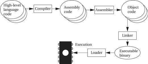
Figure 5.10 Program generation from compilation through loading.
Absolute and relative addresses
The simplest form of the assembler assumes that the starting address of the assembly language program has been specified by the programmer. The addresses in such a program are known as absolute addresses. However, in many cases, particularly when we are creating an executable out of several component files, we do not want to specify the starting addresses for all the modules before assembly—if we did, we would have to determine before assembly not only the length of each program in memory but also the order in which they would be linked into the program. Most assemblers therefore allow us to use relative addresses by specifying at the start of the file that the origin of the assembly language module is to be computed later. Addresses within the module are then computed relative to the start of the module. The linker is then responsible for translating relative addresses into addresses.
5.4.1 Assemblers
When translating assembly code into object code, the assembler must translate opcodes and format the bits in each instruction, and translate labels into addresses. In this section, we review the translation of assembly language into binary.
Labels make the assembly process more complex, but they are the most important abstraction provided by the assembler. Labels let the programmer (a human programmer or a compiler generating assembly code) avoid worrying about the locations of instructions and data. Label processing requires making two passes through the assembly source code:
1. The first pass scans the code to determine the address of each label.
2. The second pass assembles the instructions using the label values computed in the first pass.
Symbol table
As shown in Figure 5.11, the name of each symbol and its address is stored in a symbol table that is built during the first pass. The symbol table is built by scanning from the first instruction to the last. (For the moment, we assume that we know the address of the first instruction in the program.) During scanning, the current location in memory is kept in a program location counter (PLC). Despite the similarity in name to a program counter, the PLC is not used to execute the program, only to assign memory locations to labels. For example, the PLC always makes exactly one pass through the program, whereas the program counter makes many passes over code in a loop. Thus, at the start of the first pass, the PLC is set to the program’s starting address and the assembler looks at the first line. After examining the line, the assembler updates the PLC to the next location (because ARM instructions are four bytes long, the PLC would be incremented by four) and looks at the next instruction. If the instruction begins with a label, a new entry is made in the symbol table, which includes the label name and its value. The value of the label is equal to the current value of the PLC. At the end of the first pass, the assembler rewinds to the beginning of the assembly language file to make the second pass. During the second pass, when a label name is found, the label is looked up in the symbol table and its value substituted into the appropriate place in the instruction.

Figure 5.11 Symbol table processing during assembly.
But how do we know the starting value of the PLC? The simplest case is addressing. In this case, one of the first statements in the assembly language program is a pseudo-op that specifies the origin of the program, that is, the location of the first address in the program. A common name for this pseudo-op (e.g., the one used for the ARM) is the ORG statement
ORG 2000
which puts the start of the program at location 2000. This pseudo-op accomplishes this by setting the PLC’s value to its argument’s value, 2000 in this case. Assemblers generally allow a program to have many ORG statements in case instructions or data must be spread around various spots in memory.
Example 5.1 illustrates the use of the PLC in generating the symbol table.
Example 5.1 Generating a Symbol Table
Let’s use the following simple example of ARM assembly code:
ORG 100
label1 ADR r4,c
LDR r0,[r4]
label2 ADR r4,d
LDR r1,[r4]
label3 SUB r0,r0,r1
The initial ORG statement tells us the starting address of the program. To begin, let’s initialize the symbol table to an empty state and put the PLC at the initial ORG statement.
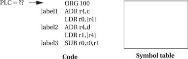
The PLC value shown is at the beginning of this step, before we have processed the ORG statement. The ORG tells us to set the PLC value to 100.
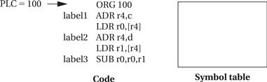
To process the next statement, we move the PLC to point to the next statement. But because the last statement was a pseudo-op that generates no memory values, the PLC value remains at 100.

Because there is a label in this statement, we add it to the symbol table, taking its value from the current PLC value.
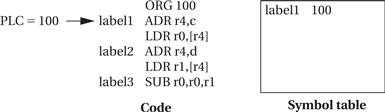
To process the next statement, we advance the PLC to point to the next line of the program and increment its value by the length in memory of the last line, namely, 4.

We continue this process as we scan the program until we reach the end, at which the state of the PLC and symbol table are as shown below.

Assemblers allow labels to be added to the symbol table without occupying space in the program memory. A typical name of this pseudo-op is EQU for equate. For example, in the code
ADD r0,r1,r2
FOO EQU 5
BAZ SUB r3,r4,#FOO
the EQU pseudo-op adds a label named FOO with the value 5 to the symbol table. The value of the BAZ label is the same as if the EQU pseudo-op were not present, because EQU does not advance the PLC. The new label is used in the subsequent SUB instruction as the name for a constant. EQUs can be used to define symbolic values to help make the assembly code more structured.
ARM ADR pseudo-op
The ARM assembler supports one pseudo-op that is particular to the ARM instruction set. In other architectures, an address would be loaded into a register (e.g., for an indirect access) by reading it from a memory location. ARM does not have an instruction that can load an effective address, so the assembler supplies the ADR pseudo-op to create the address in the register. It does so by using ADD or SUB instructions to generate the address. The address to be loaded can be register relative, program relative, or numeric, but it must assemble to a single instruction. More complicated address calculations must be explicitly programmed.
Object code formats
The assembler produces an object file that describes the instructions and data in binary format. A commonly used object file format, originally developed for Unix but now used in other environments as well, is known as COFF (common object file format). The object file must describe the instructions, data, and any addressing information and also usually carries along the symbol table for later use in debugging.
Generating relative code rather than code introduces some new challenges to the assembly language process. Rather than using an ORG statement to provide the starting address, the assembly code uses a pseudo-op to indicate that the code is in fact relocatable. (Relative code is the default for the ARM assembler.) Similarly, we must mark the output object file as being relative code. We can initialize the PLC to 0 to denote that addresses are relative to the start of the file. However, when we generate code that makes use of those labels, we must be careful, because we do not yet know the actual value that must be put into the bits. We must instead generate relocatable code. We use extra bits in the object file format to mark the relevant fields as relocatable and then insert the label’s relative value into the field. The linker must therefore modify the generated code—when it finds a field marked as relative, it uses the addresses that it has generated to replace the relative value with a correct, value for the address. To understand the details of turning relocatable code into executable code, we must understand the linking process described in the next section.
5.4.2 Linking
Many assembly language programs are written as several smaller pieces rather than as a single large file. Breaking a large program into smaller files helps delineate program modularity. If the program uses library routines, those will already be preassembled, and assembly language source code for the libraries may not be available for purchase. A linker allows a program to be stitched together out of several smaller pieces. The linker operates on the object files created by the assembler and modifies the assembled code to make the necessary links between files.
Some labels will be both defined and used in the same file. Other labels will be defined in a single file but used elsewhere as illustrated in Figure 5.12. The place in the file where a label is defined is known as an entry point. The place in the file where the label is used is called an external reference. The main job of the loader is to resolve external references based on available entry points. As a result of the need to know how definitions and references connect, the assembler passes to the linker not only the object file but also the symbol table. Even if the entire symbol table is not kept for later debugging purposes, it must at least pass the entry points. External references are identified in the object code by their relative symbol identifiers.
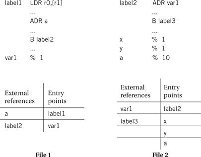
Figure 5.12 External references and entry points.
Linking process
The linker proceeds in two phases. First, it determines the address of the start of each object file. The order in which object files are to be loaded is given by the user, either by specifying parameters when the loader is run or by creating a load map file that gives the order in which files are to be placed in memory. Given the order in which files are to be placed in memory and the length of each object file, it is easy to compute the starting address of each file. At the start of the second phase, the loader merges all symbol tables from the object files into a single, large table. It then edits the object files to change relative addresses into addresses. This is typically performed by having the assembler write extra bits into the object file to identify the instructions and fields that refer to labels. If a label cannot be found in the merged symbol table, it is undefined and an error message is sent to the user.
Controlling where code modules are loaded into memory is important in embedded systems. Some data structures and instructions, such as those used to manage interrupts, must be put at precise memory locations for them to work. In other cases, different types of memory may be installed at different address ranges. For example, if we have flash in some locations and DRAM in others, we want to make sure that locations to be written are put in the DRAM locations.
Dynamically linked libraries
Workstations and PCs provide dynamically linked libraries, and certain sophisticated embedded computing environments may provide them as well. Rather than link a separate copy of commonly used routines such as I/O to every executable program on the system, dynamically linked libraries allow them to be linked in at the start of program execution. A brief linking process is run just before execution of the program begins; the dynamic linker uses code libraries to link in the required routines. This not only saves storage space but also allows programs that use those libraries to be easily updated. However, it does introduce a delay before the program starts executing.
5.4.3 Object Code Design
We have to take several issues into account when designing object code. In a timesharing system, many of these details are taken care of for us. When designing an embedded system, we may need to handle some of them ourselves.
Memory map design
As we saw, the linker allows us to control where object code modules are placed in memory. We may need to control the placement of several types of data:
• Interrupt vectors and other information for I/O devices must be placed in specific locations.
• Memory management tables must be set up.
• Global variables used for communication between processes must be put in locations that are accessible to all the users of that data.
We can give these locations symbolic names so that, for example, the same software can work on different processors that put these items at different addresses. But the linker must be given the proper absolute addresses to configure the program’s memory.
Reentrancy
Many programs should be designed to be reentrant. A program is reentrant if can be interrupted by another call to the function without changing the results of either call. If the program changes the value of global variables, it may give a different answer when it is called recursively. Consider this code:
int foo = 1;
int task1() {
foo = foo + 1;
return foo;
}
In this simple example, the variable foo is modified and so task1() gives a different answer on every invocation. We can avoid this problem by passing foo in as an argument:
int task1(int foo) {
return foo+1;
}
Relocatability
A program is relocatable if it can be executed when loaded into different parts of memory. Relocatability requires some sort of support from hardware that provides address calculation. But it is possible to write nonrelocatable code for nonrelocatable architectures. In some cases, it may be necessary to use a nonrelocatable address, such as when addressing an I/O device. However, any addresses that are not fixed by the architecture or system configuration should be accessed using relocatable code.