
6.7 Evaluating Operating System Performance
The scheduling policy does not tell us all that we would like to know about the performance of a real system running processes. Our analysis of scheduling policies makes some simplifying assumptions:
• We have assumed that context switches require zero time. Although it is often reasonable to neglect context switch time when it is much smaller than the process execution time, context switching can add significant delay in some cases.
• We have largely ignored interrupts. The latency from when an interrupt is requested to when the device’s service is complete is a critical parameter of real-time performance.
• We have assumed that we know the execution time of the processes. In fact, we learned in Section 5.7 that program time is not a single number, but can be bounded by worst-case and best-case execution times.
• We probably determined worst-case or best-case times for the processes in isolation. But, in fact, they interact with each other in the cache. Cache conflicts among processes can drastically degrade process execution time.
We need to examine the validity of all these assumptions.
Context switching time
Context switching time depends on several factors:
The execution time of the scheduler can of course be affected by coding practices. However, the choice of scheduling policy also affects the time required by the schedule to determine the next process to run. We can classify scheduling complexity as a function of the number of tasks to be scheduled. For example, round-robin scheduling, although it doesn’t guarantee deadline satisfaction, is a constant-time algorithm whose execution time is independent of the number of processes. Round-robin is often referred to as an O (1) scheduling algorithm because its execution time is a constant independent of the number of tasks. Earliest deadline first scheduling, in contrast, requires sorting deadlines, which is an O (n log n) activity.
Interrupt latency
Interrupt latency for an RTOS is the duration of time from the assertion of a device interrupt to the completion of the device’s requested operation. In contrast, when we discussed CPU interrupt latency, we were concerned only with the time the hardware took to start execution of the interrupt handler. Interrupt latency is critical because data may be lost when an interrupt is not serviced in a timely fashion.
Figure 6.17 shows a sequence diagram for RTOS interrupt latency. A task is interrupted by a device. The interrupt goes to the kernel, which may need to finish a protected operation. Once the kernel can process the interrupt, it calls the interrupt service routine (ISR), which performs the required operations on the device. Once the ISR is done, the task can resume execution.
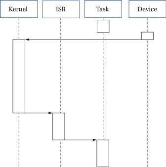
Figure 6.17 Sequence diagram for RTOS interrupt latency.
Several factors in both hardware and software affect interrupt latency:
The processor interrupt latency was chosen when the hardware platform was selected; this is often not the dominant factor in overall latency. The execution time of the handler depends on the device operation required, assuming that the interrupt handler code is not poorly designed. This leaves RTOS scheduling delays, which can be the dominant component of RTOS interrupt latency, particularly if the operating system was not designed for low interrupt latency.
Critical sections and interrupt latency
The RTOS can delay the execution of an interrupt handler in two ways. First, critical sections in the kernel will prevent the RTOS from taking interrupts. A critical section may not be interrupted, so the semaphore code must turn off interrupts. Some operating systems have very long critical sections that disable interrupt handling for very long periods. Linux is an example of this phenomenon—Linux was not originally designed for real-time operation and interrupt latency was not a major concern. Longer critical sections can improve performance for some types of workloads because it reduces the number of context switches. However, long critical sections cause major problems for interrupts.
Figure 6.18 shows the effect of critical sections on interrupt latency. If a device interrupts during a critical section, that critical section must finish before the kernel can handle the interrupt. The longer the critical section, the greater the potential delay. Critical sections are one important source of scheduling jitter because a device may interrupt at different points in the execution of processes and hit critical sections at different points.
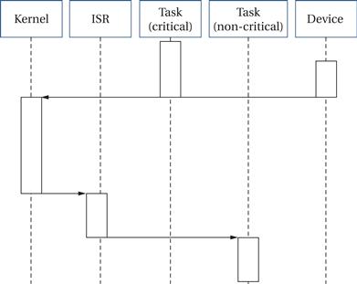
Figure 6.18 Interrupt latency during a critical section.
Interrupt priorities and interrupt latency
Second, a higher-priority interrupt may delay a lower-priority interrupt. A hardware interrupt handler runs as part of the kernel, not as a user thread. The priorities for interrupts are determined by hardware, not the RTOS. Furthermore, any interrupt handler preempts all user threads because interrupts are part of the CPU’s fundamental operation. We can reduce the effects of hardware preemption by dividing interrupt handling into two different pieces of code. First, a very simple piece of code usually called an interrupt service handler (ISH) performs the minimal operations required to respond to the device. The rest of the required processing, which may include updating user buffers or other more complex operations, is performed by a user-mode thread known as an interrupt service routine (ISR). Because the ISR runs as a thread, the RTOS can use its standard policies to ensure that all the tasks in the system receive their required resources.
RTOS performance evaluation tools
Some RTOSs provide simulators or other tools that allow you to view the operation of the processes in the system. These tools will show not only abstract events such as processes but also context switching time, interrupt response time, and other overheads. This sort of view can be helpful in both functional and performance debugging. Windows CE provides several performance analysis tools: ILTiming, an instrumentation routine in the kernel that measures both interrupt service routine and interrupt service thread latency; OSBench measures the timing of operating system tasks such as critical section access, signals, and so on; Kernel Tracker provides a graphical user interface for RTOS events.
Caches and RTOS performance
Many real-time systems have been designed based on the assumption that there is no cache present, even though one actually exists. This grossly conservative assumption is made because the system architects lack tools that permit them to analyze the effect of caching. Because they do not know where caching will cause problems, they are forced to retreat to the simplifying assumption that there is no cache. The result is extremely overdesigned hardware, which has much more computational power than is necessary. However, just as experience tells us that a well-designed cache provides significant performance benefits for a single program, a properly sized cache can allow a microprocessor to run a set of processes much more quickly. By analyzing the effects of the cache, we can make much better use of the available hardware.
Li and Wolf [Li99] developed a model for estimating the performance of multiple processes sharing a cache. In the model, some processes can be given reservations in the cache, such that only a particular process can inhabit a reserved section of the cache; other processes are left to share the cache. We generally want to use cache partitions only for performance-critical processes because cache reservations are wasteful of limited cache space. Performance is estimated by constructing a schedule, taking into account not just execution time of the processes but also the state of the cache. Each process in the shared section of the cache is modeled by a binary variable: 1 if present in the cache and 0 if not. Each process is also characterized by three total execution times: assuming no caching, with typical caching, and with all code always resident in the cache. The always-resident time is unrealistically optimistic, but it can be used to find a lower bound on the required schedule time. During construction of the schedule, we can look at the current cache state to see whether the no-cache or typical-caching execution time should be used at this point in the schedule. We can also update the cache state if the cache is needed for another process. Although this model is simple, it provides much more realistic performance estimates than assuming the cache either is nonexistent or is perfect. Example 6.8 shows how cache management can improve CPU utilization.
Example 6.8 Effects of Scheduling on the Cache
Consider a system containing the following three processes:
| Process | Worst-case CPU time | Average-case CPU time |
| P1 | 8 | 6 |
| P2 | 4 | 3 |
| P3 | 4 | 3 |
Each process uses half the cache, so only two processes can be in the cache at the same time.
Appearing below is a first schedule that uses a least-recently-used cache replacement policy on a process-by-process basis.
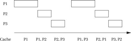
In the first iteration, we must fill up the cache, but even in subsequent iterations, competition among all three processes ensures that a process is never in the cache when it starts to execute. As a result, we must always use the worst-case execution time.
Another schedule in which we have reserved half the cache for P1 is shown below. This leaves P2 and P3 to fight over the other half of the cache.
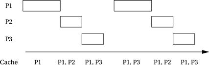
In this case, P2 and P3 still compete, but P1 is always ready. After the first iteration, we can use the average-case execution time for P1, which gives us some spare CPU time that could be used for additional operations.