
5.2 Components for Embedded Programs
In this section, we consider code for three structures or components that are commonly used in embedded software: the state machine, the circular buffer, and the queue. State machines are well suited to reactive systems such as user interfaces; circular buffers and queues are useful in digital signal processing.
5.2.1 State Machines
State machine style
When inputs appear intermittently rather than as periodic samples, it is often convenient to think of the system as reacting to those inputs. The reaction of most systems can be characterized in terms of the input received and the current state of the system. This leads naturally to a finite-state machine style of describing the reactive system’s behavior. Moreover, if the behavior is specified in that way, it is natural to write the program implementing that behavior in a state machine style. The state machine style of programming is also an efficient implementation of such computations. Finite-state machines are usually first encountered in the context of hardware design.
Programming Example 5.1 shows how to write a finite-state machine in a high-level programming language.
Programming Example 5.1 A State Machine in C
The behavior we want to implement is a simple seat belt controller [Chi94]. The controller’s job is to turn on a buzzer if a person sits in a seat and does not fasten the seat belt within a fixed amount of time. This system has three inputs and one output. The inputs are a sensor for the seat to know when a person has sat down, a seat belt sensor that tells when the belt is fastened, and a timer that goes off when the required time interval has elapsed. The output is the buzzer. Appearing below is a state diagram that describes the seat belt controller’s behavior.

The idle state is in force when there is no person in the seat. When the person sits down, the machine goes into the seated state and turns on the timer. If the timer goes off before the seat belt is fastened, the machine goes into the buzzer state. If the seat belt goes on first, it enters the belted state. When the person leaves the seat, the machine goes back to idle.
To write this behavior in C, we will assume that we have loaded the current values of all three inputs (seat, belt, timer) into variables and will similarly hold the outputs in variables temporarily (timer_on, buzzer_on). We will use a variable named state to hold the current state of the machine and a switch statement to determine what action to take in each state. Here is the code:
#define IDLE 0
#define SEATED 1
#define BELTED 2
#define BUZZER 3
switch(state) { /* check the current state */
case IDLE:
if (seat){ state = SEATED; timer_on = TRUE; }
/* default case is self-loop */
break;
case SEATED:
if (belt) state = BELTED; /* won’t hear the buzzer */
else if (timer) state = BUZZER; /* didn’t put on belt in time */
/* default case is self-loop */
break;
case BELTED:
if (!seat) state = IDLE; /* person left */
else if (!belt) state = SEATED; /* person still in seat */
break;
case BUZZER:
if (belt) state = BELTED; /* belt is on---turn off buzzer */
else if (!seat) state = IDLE; /* no one in seat--turn off buzzer */
break;
}
This code takes advantage of the fact that the state will remain the same unless explicitly changed; this makes self-loops back to the same state easy to implement. This state machine may be executed forever in a while(TRUE) loop or periodically called by some other code. In either case, the code must be executed regularly so that it can check on the current value of the inputs and, if necessary, go into a new state.
5.2.2 Circular Buffers and Stream-Oriented Programming
Data stream style
The data stream style makes sense for data that comes in regularly and must be processed on the fly. The FIR filter of Application Example 2.1 is a classic example of stream-oriented processing. For each sample, the filter must emit one output that depends on the values of the last n inputs. In a typical workstation application, we would process the samples over a given interval by reading them all in from a file and then computing the results all at once in a batch process. In an embedded system we must not only emit outputs in real time, but we must also do so using a minimum amount of memory.
Circular buffer
The circular buffer is a data structure that lets us handle streaming data in an efficient way. Figure 5.1 illustrates how a circular buffer stores a subset of the data stream. At each point in time, the algorithm needs a subset of the data stream that forms a window into the stream. The window slides with time as we throw out old values no longer needed and add new values. Because the size of the window does not change, we can use a fixed-size buffer to hold the current data. To avoid constantly copying data within the buffer, we will move the head of the buffer in time. The buffer points to the location at which the next sample will be placed; every time we add a sample, we automatically overwrite the oldest sample, which is the one that needs to be thrown out. When the pointer gets to the end of the buffer, it wraps around to the top.

Figure 5.1 A circular buffer.
Instruction set support
Many DSPs provide addressing modes to support circular buffers. For example, the C55x [Tex04] provides five circular buffer start address registers (their names start with BSA). These registers allow circular buffers to be placed without alignment constraints.
In the absence of specialized instructions, we can write our own C code for a circular buffer. This code also helps us understand the operation of the buffer. Programming Example 5.2 provides an efficient implementation of a circular buffer.
High-level language implementation
Programming Example 5.2 A Circular Buffer in C
Once we build a circular buffer, we can use it in a variety of ways. We will use an array as the buffer:
#define CMAX 6 /* filter order */
int circ[CMAX]; /* circular buffer */
int pos; /* position of current sample */
The variable pos holds the position of the current sample. As we add new values to the buffer this variable moves.
Here is the function that adds a new value to the buffer:
void circ_update(int xnew) {
/* add the new sample and push off the oldest one */
/* compute the new head value with wraparound; the pos pointer moves from 0 to CMAX-1 */
pos = ((pos == CMAX-1) ? 0 : (pos+1));
/* insert the new value at the new head */
circ[pos] = xnew;
}
The assignment to pos takes care of wraparound—when pos hits the end of the array it returns to zero. We then put the new value into the buffer at the new position. This overwrites the old value that was there. Note that as we go to higher index values in the array we march through the older values.
We can now write an initialization function. It sets the buffer values to zero. More important, it sets pos to the initial value. For ease of debugging, we want the first data element to go into circ[0]. To do this, we set pos to the end of the array so that it is set to zero before the first element is added:
void circ_init() {
int i;
for (i=0; i<CMAX; i++) /* set values to 0 */
circ[i] = 0;
pos=CMAX-1; /* start at tail so first element will be at 0 */
}
We can also make use of a function to get the ith value of the buffer. This function has to translate the index in temporal order—zero being the newest value—to its position in the array:
int circ_get(int i) {
/* get the ith value from the circular buffer */
int ii;
/* compute the buffer position */
ii = (pos - i) % CMAX;
/* return the value */
return circ[ii];
}
We are now in a position to write C code for a digital filter. To help us understand the filter algorithm, we can introduce a widely used representation for filter functions.
Signal flow graph
The FIR filter is only one type of digital filter. We can represent many different filtering structures using a signal flow graph as shown in Figure 5.2. The filter operates at a sample rate with inputs arriving and outputs generated at the sample rate. The inputs x[n] and y[n] are sequences indexed by n, which corresponds to the sequence of samples. Nodes in the graph can represent either arithmetic operators or delay operators. The + node adds its two inputs and produces the output y[n]. The box labeled z-1 is a delay operator. The z notation comes from the z transform used in digital signal processing; the −1 superscript means that the operation performs a time delay of one sample period. The edge from the delay operator to the addition operator is labeled with b1, meaning that the output of the delay operator is multiplied by b1.
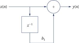
Figure 5.2 A signal flow graph.
Filters and buffering
The code to produce one FIR filter output looks like this:
for (i=0, y=0.0; i<N; i++)
y += x[i] * b[i];
However, the filter takes in a new sample on every sample period. The new input becomes x1 , the old x1 becomes x2 , etc. x0 is stored directly in the circular buffer but must be multiplied by b0 before being added to the output sum. Early digital filters were built-in hardware, where we can build a shift register to perform this operation. If we used an analogous operation in software, we would move every value in the filter on every sample period. We can avoid that with a circular buffer, moving the head without moving the data elements.
The next example uses our circular buffer class to build an FIR filter.
Programming Example 5.3 An FIR Filter in C
Here is a signal flow graph for an FIR filter:
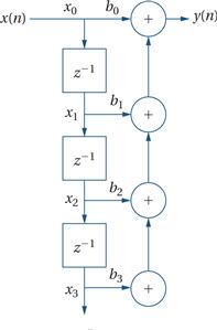
The delay elements running vertically hold the input samples with the most recent sample at the top and the oldest one at the bottom. Unfortunately, the signal flow graph doesn’t explicitly label all of the values that we use as inputs to operations, so the figure also shows the values (xi ) we need to operate on in our FIR loop.
When we compute the filter function, we want to match the bi’s and xi’s. We will use our circular buffer for the x’s, which change over time. We will use a standard array for the b’s, which don’t change. In order for the filter function to be able to use the same I value for both sets of data, we need to put the x data in the proper order. We can put the b data in a standard array with b0 being the first element. When we add a new x value, it becomes x![]() 0 and replaces the oldest data value in the buffer. This means that the buffer head moves from higher to lower values, not lower to higher as we might expect.
0 and replaces the oldest data value in the buffer. This means that the buffer head moves from higher to lower values, not lower to higher as we might expect.
Here is the modified version of circ_update() that puts a new sample into the buffer into the desired order:
void circ_update(int xnew) {
/* add the new sample and push off the oldest one */
/* compute the new head value with wraparound; the pos pointer moves from CMAX-1 down to 0 */
pos = ((pos == 0) ? CMAX-1 : (pos-1));
/* insert the new value at the new head */
circ[pos] = xnew;
}
We also need to change circ_init() to set pos = 0 initially. We don’t need to change circ_get();
Given these functions, the filter itself is simple. Here is our code for the FIR filter function:
int fir(int xnew) {
/* given a new sample value, update the queue and compute the filter output */
int i;
int result; /* holds the filter output */
circ_update(xnew); /* put the new value in */
for (i=0, result=0; i<CMAX; i++) /* compute the filter function */
result += b[i] * circ_get(i);
return result;
}
There is only one major structure for FIR filters but several for IIR filters, depending on the application requirements. One of the important reasons for so many different IIR forms is numerical properties—depending on the filter structure and coefficients, one structure may give significantly less numerical noise than another. But numerical noise is beyond the scope of our discussion so let’s concentrate on one form of IIR filter that highlights buffering issues. The next example looks at one form of IIR filter.
Programming Example 5.4 A Direct Form II IIR Filter Class in C
Here is what is known as the direct form II of an IIR filter:

This structure is designed to minimize the amount of buffer space required. Other forms of the IIR filter have other advantages but require more storage. We will store the vi values as in the FIR filter. In this case, v0 does not represent the input, but rather the left-hand sum. But v0 is stored before multiplication by b0 so that we can move v0 to v1 on the following sample period.
We can use the same circ_update() and circ_get() functions that we used for the FIR filter. We need two coefficient arrays, one for as and one for bs; as with the FIR filter, we can use standard C arrays for the coefficients because they don’t change over time. Here is the IIR filter function:
int iir2(int xnew) {
/* given a new sample value, update the queue and compute the filter output */
int i, aside, bside, result;
for (i=0, aside=0; i<ZMAX; i++)
aside += -a[i+1] * circ_get(i);
for (i=0, bside=0; i<ZMAX; i++)
bside += b[i+1] * circ_get(i);
result = b[0] * (xnew + aside) + bside;
circ_update(xnew); /* put the new value in */
return result;
}
5.2.3 Queues and Producer/Consumer Systems
Queues are also used in signal processing and event processing. Queues are used whenever data may arrive and depart at somewhat unpredictable times or when variable amounts of data may arrive. A queue is often referred to as an elastic buffer. We saw how to use elastic buffers for I/O in Chapter 3.
One way to build a queue is with a linked list. This approach allows the queue to grow to an arbitrary size. But in many applications we are unwilling to pay the price of dynamically allocating memory. Another way to design the queue is to use an array to hold all the data. Although some writers use both circular buffer and queue to mean the same thing, we use the term circular buffer to refer to a buffer that always has a fixed number of data elements while a queue may have varying numbers of elements in it.
Programming Example 5.5 gives C code for a queue that is built from an array.
Programming Example 5.5 An Array-Based Queue
The first step in designing the queue is to declare the array that we will use for the buffer:
#define Q_SIZE 5 /* your queue size may vary */
#define Q_MAX (Q_SIZE-1) /* this is the maximum index value into the array */
int q[Q_SIZE]; /* the array for our queue */
int head, tail; /* indexes for the current queue head and tail */
The variables head and tail keep track of the two ends of the queue.
Here is the initialization code for the queue:
void queue_init() {
/* initialize the queue data structure */
head = 0;
tail = 0;
}
We initialize the head and tail to the same position. As we add a value to the tail of the queue, we will increment tail. Similarly, when we remove a value from the head, we will increment head. The value of head is always equal to the location of the first element of the queue (except for when the queue is empty). The value of tail, in contrast, points to the location in which the next queue entry will go. When we reach the end of the array, we must wrap around these values—for example, when we add a value into the last element of q, the new value of tail becomes the 0th entry of the array.
We need to check for two error conditions: removing from an empty queue and adding to a full queue. In the first case, we know the queue is empty if head == tail. In the second case, we know the queue is full if incrementing tail will cause it to equal head. Testing for fullness, however, is a little harder because we have to worry about wraparound.
Here is the code for adding an element to the tail of the queue, which is known as enqueueing:
void enqueue(int val) {
/* check for a full queue */
if (((tail+1) % Q_SIZE) == head) error("enqueue onto full queue",tail);
/* add val to the tail of the queue */
q[tail] = val;
/* update the tail */
if (tail == Q_MAX)
tail = 0;
else
tail++;
}
And here is the code for removing an element from the head of the queue, known as dequeueing:
int dequeue() {
int returnval; /* use this to remember the value that you will return */
/* check for an empty queue */
if (head == tail) error("dequeue from empty queue",head);
/* remove from the head of the queue */
returnval = q[head];
/* update head */
if (head == Q_MAX)
head = 0;
else
head++;
/* return the value */
return returnval;
}
Digital filters always take in the same amount of data in each time period. Many systems, even signal processing systems, don’t fit that mold. Rather, they may take in varying amounts of data over time and produce varying amounts. When several of these systems operate in a chain, the variable-rate output of one stage becomes the variable-rate input of another stage.
Producer/consumer
Figure 5.3 shows a block diagram of a simple producer/consumer system. p1 and p2 are the two blocks that perform algorithmic processing. The data is fed to them by queues that act as elastic buffers. The queues modify the flow of control in the system as well as store data. If, for example, p2 runs ahead of p1, it will eventually run out of data in its q12 input queue. At that point, the queue will return an empty signal to p2. At this point, p2 should stop working until more data is available. This sort of complex control is easier to implement in a multitasking environment, as we will see in Chapter 6, but it is also possible to make effective use of queues in programs structured as nested procedures.

Figure 5.3 A producer/consumer system.
Data structures in queues
The queues in a producer/consumer may hold either uniform-sized data elements or variable-sized data elements. In some cases, the consumer needs to know how many of a given type of data element are associated together. The queue can be structured to hold a complex data type. Alternatively, the data structure can be stored as bytes or integers in the queue with, for example, the first integer holding the number of successive data elements.