CHAPTER 5
Index Futures
Aims
- To provide details of contract specification, settlement procedures and quotes for stock index futures contracts.
- To demonstrate index arbitrage and program trading using stock index futures.
- To price a stock index futures contract, when stocks which make up the cash market index (e.g. S&P 500), pay discrete dividends.
- To determine the number of futures contracts to use when hedging various cash market positions (e.g. a portfolio of stocks or holding barrels of oil).
- To outline the risks which remain, after hedging with index futures.
- To demonstrate ‘tailing the hedge’.
Stock index futures (SIF) are contracts whose price depends on an underlying stock market index such as the S&P 500, FTSE 100 or Nikkei 225 indices. Such futures contracts are widely used in hedging, speculation, and index arbitrage.
In a well-diversified portfolio of stocks, specific (idiosyncratic) risk of individual stocks has been largely eliminated and only ‘market’ (‘systematic’ or ‘non-diversifiable’) risk remains. Stock index futures can be used to eliminate this ‘market risk’ of the portfolio of stocks. In ‘normal times’ a fund manager might be quite happy to hold a diversified portfolio of stocks even though they are risky. But if a fund manager believes the market will become increasingly volatile over the next 3 months (i.e. could rise or fall substantially) and she wished to remove this uncertainty, she could sell stock index futures to eliminate the market risk. At the end of the 3-month period, she would have neither gained nor lost.1 If she believes the stock market has then returned to a ‘normal level of volatility’, she would close out her futures position and her stock portfolio would again be subject to market risk.
Alternatively, suppose you plan to invest cash that you will receive in 3 months' time in a diversified portfolio of stocks but you are worried that the stock market will rise over the next 3 months. By buying stock index futures today you can fix the effective future purchase price of the stocks.
Also, speculation on a bear or bull market is easier to achieve with stock index futures rather than incurring the cost of buying or selling a large number of stocks that make up your prospective speculative stock portfolio. Finally, if the quoted stock index futures price is not equal to the ‘correct’ (no arbitrage) futures price then you can make a (near) risk-free arbitrage profit by simultaneously trading in the spot and futures markets. We elaborate on these ideas in this chapter and consider further strategies in later chapters.
5.1 STOCK INDEX FUTURES (SIF)
Stock index futures contracts are written on aggregate stock market indices and are settled in cash. In the US index futures contracts traded on the CME (Chicago) include those on the S&P 500, the Mini-S&P 500, the Russel 1000 (large cap index), the Dow Jones Industrial Average (DJIA) and the Nikkei 225 (Japanese index), as well as several other indices. Trading volume is highest in the S&P 500 futures contract and taking all of these contracts together, the dollar volume of the underlying stocks traded in these index futures contracts exceeds the dollar volume on the stock market itself.
On LIFFE2 (pronounced ‘life’), futures contracts are available on various UK stock indices including the FTSE 100 and FTSE 250 indices, on European indices such as the FTSE Eurotop 100 and FTSE Eurotop 300 (including and excluding the UK), and several others. The reason for so many different index futures contracts is so that fund managers can effectively hedge their existing equity portfolios, using a futures contract which has an underlying stock index that most closely matches the composition of their own cash market stock portfolio. Details of some of these contracts are given in Table 5.1.
TABLE 5.1 Stock index futures contract
| FTSE 100 | S&P 500 | FTSE Eurotop 300 | Nikkei 225 | DJIA | |
| Unit of trading | £10 × index | $250 × index | €20 × index | $5 × index | $10 × index |
| Expiration | Mar/Jun/Sep/Dec | Mar/Jun/Sep/Dec | Mar/Jun/Sep/Dec | Mar/Jun/Sep/Dec | Mar/Jun/Sep/Dec |
| Exchange | NYSE-Euronext | CME Group (IMM) | NYSE-Euronext | CME Group (IMM) | CME Group (IMM) |
5.1.1 Contract Multiple
All stock index futures are settled in cash (with settlement procedures differing between the different contracts) and nearly all contracts are closed out prior to their maturity date. Cash settlement is based on the value of an index point $z (or the ‘contract multiple’), which is set by the exchange (for the S&P 500, ![]() ). For the S&P 500 index futures contract, the smallest price change, a tick, is 0.1 index points, representing a $25 change in value of one futures contract. Hence, a 1-point change in the S&P 500 futures index implies a change in the dollar value of one futures contract of $250. If the futures index on the S&P 500 is currently F0 = 2000, then:
). For the S&P 500 index futures contract, the smallest price change, a tick, is 0.1 index points, representing a $25 change in value of one futures contract. Hence, a 1-point change in the S&P 500 futures index implies a change in the dollar value of one futures contract of $250. If the futures index on the S&P 500 is currently F0 = 2000, then:
5.1.2 Stock Indices
The S&P 500 and FTSE 100 stock indices are value (market capitalisation) weighted indices. The S&P 500 and FTSE 100 indices ignore dividend payments and therefore do not truly reflect the ‘total returns’ from the constituent shares (which include dividend payments). Often a stock index will have both a ‘price version’ and a ‘total return’ version.
5.1.3 Newspaper Quotes
Newspaper quotes for different stock index futures contracts are very similar. An illustrative example of price quotes (on 27 July) for futures contracts on the S&P 500 (traded on CME) with different maturities are given in Table 5.2.
TABLE 5.2 Quotes, index futures (27 July)
| S&P 500 Index Futures (CME) | ||||||
| Open | Settle | Change | High | Low | Open interest | |
| September | 2,484.60 | 2,469.00 | –15.50 | 2,485.20 | 2,466.00 | 677,803 |
| December | 2,499.00 | 2,491.30 | –15.70 | 2,503.00 | 2,490.00 | 17,481 |
| March | 2,520.20 | 2,513.30 | –16.20 | 2,526.00 | 2,514.00 | 1,094 |
| June | 2,537.20 | 2,561.80 | –16.20 | 2,549.50 | 2,537.20 | 929 |
| September | 2,562.20 | 2,561.80 | –16.30 | 2,574.10 | 2,562.10 | 146 |
The settlement price (‘Settle’) is an average of futures prices for trades at the end of the trading day – the settlement price is used in ‘marking-to-market’ and establishing margin payments. ‘Open interest’ is the number of contracts held (long or short) and is highest for the nearby September index futures contract and tails off rapidly for longer maturity contracts. Note that for S&P 500 futures contracts, the longer maturity contracts have higher quoted settlement prices today, than the nearby maturing contracts (see the ‘Settle’ column, Table 5.2). There are also index futures available on many other stock indices (e.g. on US ‘high tech’ stocks in the NASDAQ-100 (CME); the CAC-40 French stock index (traded in Paris on the MATIF exchange), and the DAX-30 German index (traded on the EUREX exchange in Frankfurt).
5.2 INDEX ARBITRAGE
In Chapter 3 we used ‘cash-and-carry arbitrage’ to derive the correct (fair, no-arbitrage) futures price on a stock, which also applies to the futures price on a stock index:
where
| S | = | S&P 500 stock index (quoted on the NYSE) |
| F | = | S&P 500 futures index (quoted in Chicago) |
| T | = | time to maturity of the futures contract, number of years (or fraction of a year) |
| r | = | (domestic) risk-free interest rate (proportionate, p.a.) |
| δ | = | dividend yield (proportionate, p.a) |
If the current risk-free rate ![]() is greater than the dividend yield (i.e.
is greater than the dividend yield (i.e. ![]() ) then the current quoted futures price (in Chicago) will be above the current stock price (on the NYSE), that is
) then the current quoted futures price (in Chicago) will be above the current stock price (on the NYSE), that is ![]() , and vice versa. In applying the ‘cost-of-carry’ model we have to make the following assumptions:
, and vice versa. In applying the ‘cost-of-carry’ model we have to make the following assumptions:
- Investors can purchase or short-sell stocks, to ‘replicate’ the performance of all the stocks in the stock index.
- Actual discrete dividends paid out from stocks in the S&P 500 index (over the life of the futures) can be approximated by a constant (value weighted) dividend yield,
 , or actual discrete dividend payments from the stocks in the index are known with certainty (see below).
5.2.1 Program Trading
If the quoted futures price is not given by the equalities in (5.1), then index arbitrage enables (almost) risk-free profits to be made. In large financial institutions real time data on ![]() ,
, ![]() ,
, ![]() ,
, ![]() and the quoted futures price
and the quoted futures price ![]() are fed into computers and when
are fed into computers and when ![]() in Equation (5.1), an arbitrage strategy is applied.
in Equation (5.1), an arbitrage strategy is applied.
Borrowing or lending cash at ![]() to undertake the arbitrage transaction is usually done via the repo market. Suppose an arbitrageur is faced with the following data:
to undertake the arbitrage transaction is usually done via the repo market. Suppose an arbitrageur is faced with the following data:

‘Fair’ futures price:
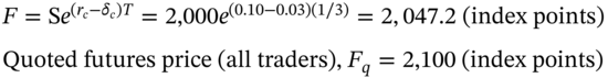
The quoted futures price ![]() is above the fair futures price
is above the fair futures price ![]() , so an arbitrage opportunity (i.e. ‘sell high, buy low’) is possible. You sell the futures contract today at
, so an arbitrage opportunity (i.e. ‘sell high, buy low’) is possible. You sell the futures contract today at ![]() , borrow
, borrow ![]() at
at ![]() for 4 months (T = 1/3) and purchase the underlying stocks today.3 After receiving dividend payments at the (continuously compounded) rate
for 4 months (T = 1/3) and purchase the underlying stocks today.3 After receiving dividend payments at the (continuously compounded) rate ![]() on your stocks, you owe 2,047.2 after 4 months. You deliver the stocks against the short futures position after 4 months and receive
on your stocks, you owe 2,047.2 after 4 months. You deliver the stocks against the short futures position after 4 months and receive ![]() (in Chicago, from the long futures counterparty), making an arbitrage profit of
(in Chicago, from the long futures counterparty), making an arbitrage profit of ![]() .
.
Conversely, suppose the quoted futures price is ![]() . Today, the arbitrage strategy is to buy the futures contract ‘low’ at 2,020, simultaneously short-sell a portfolio of stocks for
. Today, the arbitrage strategy is to buy the futures contract ‘low’ at 2,020, simultaneously short-sell a portfolio of stocks for ![]() and invest the proceeds in a bank deposit at the risk-free rate. At maturity of the long futures position you pay out
and invest the proceeds in a bank deposit at the risk-free rate. At maturity of the long futures position you pay out ![]() , take delivery of the stocks (in Chicago), which you return to your broker. You also have to pay the broker any dividends due on the borrowed stocks. Hence your net receipts from investing the
, take delivery of the stocks (in Chicago), which you return to your broker. You also have to pay the broker any dividends due on the borrowed stocks. Hence your net receipts from investing the ![]() at the risk-free rate would be
at the risk-free rate would be ![]() and the arbitrage profit at T, is 27.2 (receipts of 2047.2 minus payments of 2020).
and the arbitrage profit at T, is 27.2 (receipts of 2047.2 minus payments of 2020).
5.2.2 Discrete Dividend Payments
In practice, dividend payments are clustered around certain months (particularly February and March in the US) so that the assumption of a constant dividend yield is an approximation. However, the arbitrage relationship is similar when dividends are paid in discrete amounts. Assume there are N-dividend payments of ![]() , each of which is paid
, each of which is paid ![]() years (or fraction of a year) from today
years (or fraction of a year) from today ![]() (Figure 5.1).
(Figure 5.1).
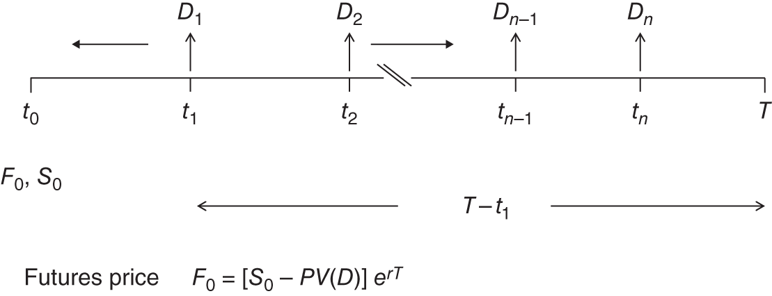
FIGURE 5.1 Futures price: dividend paying stock
All of the individual discrete dividend payments at time t = 0 are worth:
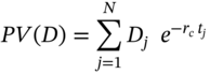
Each dividend payment ![]() payable
payable ![]() years from today is discounted, which puts all dividend payments at
years from today is discounted, which puts all dividend payments at ![]() , the same point in time as the stock price
, the same point in time as the stock price ![]() . Hence the net cost of a replication portfolio at
. Hence the net cost of a replication portfolio at ![]() is
is ![]() , which accrues to
, which accrues to ![]() at T the maturity of the futures, so today's no-arbitrage futures price is:
at T the maturity of the futures, so today's no-arbitrage futures price is:
Above we assumed ![]() is constant for all maturities (i.e. yield curve is flat over t = 0 to T) – but if not, this is easily taken care of by using
is constant for all maturities (i.e. yield curve is flat over t = 0 to T) – but if not, this is easily taken care of by using ![]() in place of
in place of ![]() .
.
There is basis risk in the arbitrage strategy for several reasons. First, traders might only buy (or sell) a subset of the 500 stocks which make up the S&P 500 index. Hence the change in value of the arbitrageur's portfolio of stocks might not exactly match the change in value of the S&P 500 stock index. Second, there are the arbitrageur's transactions costs to consider and any uncertainty in the timing of dividend payments over the life of the futures contract. Third, it might not be possible to execute trades in the index futures contract and all the stocks (in the index) at exactly the same time – in the meantime the prices of some of the underlying stocks might change.
Because index arbitrage opportunities are calculated using computerised real-time data, it is also known as program trading and is the subject of some controversy when the markets move rapidly (see Finance Blog 5.1).
Academic studies suggest that index arbitrage profits are difficult to exploit but tend to occur more often in those contracts with a longer time to maturity. This may be because these are the less liquid contracts where the ‘fair price’ and the quoted futures price might diverge because traders cannot obtain credit lines for these longer periods and therefore cannot instigate the arbitrage transaction.
Over the past few years, replicating the movement in a stock market index has been made much simpler by the introduction of Exchange Traded Funds (ETFs). These are ‘funds’ that closely track changes in a specific index and can be bought and sold (at all times of the day) in the ‘cash market’, usually on electronic platforms at low transactions costs. This means that it is nearly always the case that index arbitrage ensures that the index futures price is given by ![]() .
.
5.3 HEDGING
A well-diversified stock portfolio dramatically reduces ‘specific (idiosyncratic) risk’, while stock index futures contracts allow investors to hedge against changes in (overall stock) ‘market risk’ which is usually assumed to be adequately measured by some broad stock market index, which we take to be the S&P 500 index.
Hedging relies on the positive correlation between spot and futures prices. This implies that if you hold a portfolio of stocks (‘long in the cash market’), then shorting stock index futures contracts ‘creates’ a negative correlation – what you lose on your cash market stock portfolio, you hope to gain on your index futures position. If a hedged portfolio entirely eliminates market risk then we might expect it to earn the risk-free rate of return.
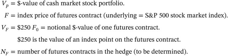
Suppose that on 28 December Ms Midas holds a $10m diversified portfolio of US stocks which exactly mirrors the composition of the S&P 500 index, so the beta of her stock portfolio ![]() . She feels the stock market is likely to be more volatile (than normal) over the next 3 months. This presents both opportunities for large price rises and large price falls. But let us assume that Ms Midas is very worried about a general fall in the stock market over the next 3 months, between 28 December and 28 March. This may be because she has already achieved the target return on her portfolio and is worried that her past gains are likely to be eroded over the next 3 months – which is the end of the period over which her performance (and bonus) will be evaluated by her superiors.
. She feels the stock market is likely to be more volatile (than normal) over the next 3 months. This presents both opportunities for large price rises and large price falls. But let us assume that Ms Midas is very worried about a general fall in the stock market over the next 3 months, between 28 December and 28 March. This may be because she has already achieved the target return on her portfolio and is worried that her past gains are likely to be eroded over the next 3 months – which is the end of the period over which her performance (and bonus) will be evaluated by her superiors.
She can use stock index futures to eliminate this market risk (and earn the risk-free rate of interest) over the 3-month period. Of course, she could also earn the risk-free rate by selling all her stocks and holding T-bills. However, this would involve high transactions costs, as she would have to sell and then buy-back the stocks 3 months later. Continuing to hold the portfolio of stocks and hedging using stock index futures is far cheaper.
To hedge over 3 months she requires a futures contract which has at least 3 months to maturity. Suppose on 28 December Ms Midas decides to use the June-futures (which has a maturity date towards the end of June). Stock index futures (on the S&P 500) are cash settled with each index point (‘tick’) on the futures contract is assigned a value of $250.
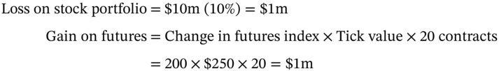
Ms Midas can hedge on 28 December by selling (shorting) the June-index futures (on the S&P 500). For the moment, assume a perfect correlation between the underlying market index S and the futures index F (i.e. correlation coefficient of +1) and that both indices move by the same amount. If the S&P 500 index on the NYSE on 28 December is ![]() and the market falls by 10% over the next 3 months, the S&P index will fall to 1,800 (i.e. by 200 points). Ms Midas's stock portfolio will fall in value by
and the market falls by 10% over the next 3 months, the S&P index will fall to 1,800 (i.e. by 200 points). Ms Midas's stock portfolio will fall in value by ![]() . If we assume F and S move by the same absolute amount then the change in
. If we assume F and S move by the same absolute amount then the change in ![]() points and the change in value of one futures contract is
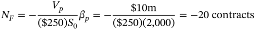
points and the change in value of one futures contract is ![]() . Hence the number of futures contracts to hedge your stock portfolio is:
. Hence the number of futures contracts to hedge your stock portfolio is:

So Ms Midas would hedge by shorting 20 contracts on 28 December. The outcome of the hedged position on 28 March is therefore:
The reader can verify that a similar hedged outcome would ensue if stock prices rise by 10%. Here, the capital gain on the stocks would be offset by the loss on the short futures position – after F increases Ms Midas has to buy back the futures at a higher price (i.e. at a loss). In this case, with hindsight it would have been better not to have hedged – but ‘hindsight’ is not ‘available’ on 28 December. In any case the whole idea of a hedge is to remove price risk and in doing so, you also forego any favourable outcomes if stock prices rise. ‘You can't have your cake and eat it’ – you can be a hedger or a speculator in any given deal, but not both.
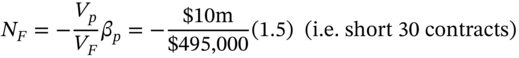
If the beta of Ms Midas's portfolio of stocks is ![]() and the market falls by 10%, the return on her portfolio falls by 15%
and the market falls by 10%, the return on her portfolio falls by 15% ![]() . Hence, she needs more futures contracts for an effective hedge. She would in fact need to short 30 futures contracts. This is because the change in the dollar value of her stock portfolio is now expected to be
. Hence, she needs more futures contracts for an effective hedge. She would in fact need to short 30 futures contracts. This is because the change in the dollar value of her stock portfolio is now expected to be ![]() , so
, so ![]() .
.
The above example looks a bit too good to be true – a perfect hedge. Yes, this is too optimistic! The reason for this is that we assumed the absolute change in the two indices, F and S are exactly the same. In practice this is not the case. First, F and S do not move exactly together, ‘index point-for-index point’ – they do so only approximately. Second, because interest rates might change over the life of the hedge, this slightly affects the relationship between changes in F and S – recall that ![]() – this is basis risk. Third, because the beta of your portfolio of stocks is estimated with error, when the market moves by 10% the value of your stock portfolio might not move by exactly 15% – this is probably the biggest source of error in the hedge.
– this is basis risk. Third, because the beta of your portfolio of stocks is estimated with error, when the market moves by 10% the value of your stock portfolio might not move by exactly 15% – this is probably the biggest source of error in the hedge.
Let's return to the case where ![]() and consider a more realistic scenario where there would be some hedging error. On 28 December the S&P 500 index
and consider a more realistic scenario where there would be some hedging error. On 28 December the S&P 500 index ![]() and the futures index price
and the futures index price ![]() . Over the next 3 months the portfolio manager's worst fears are met and the S&P 500 index falls by 10% (200 index points) to
. Over the next 3 months the portfolio manager's worst fears are met and the S&P 500 index falls by 10% (200 index points) to ![]() , so Ms Midas's stock portfolio falls in value by $1m. On 28 March, the June-futures index falls to
, so Ms Midas's stock portfolio falls in value by $1m. On 28 March, the June-futures index falls to ![]() – a fall of 222 index points4 – the futures contracts are closed out (i.e. buy-back) and the outcome of the hedged position on 28 March is:
– a fall of 222 index points4 – the futures contracts are closed out (i.e. buy-back) and the outcome of the hedged position on 28 March is:
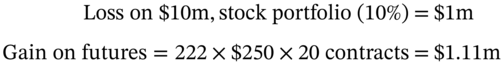
Hence the hedge position has produced a small profit of $110,000 (1.1% of the portfolio value of $10m). But most importantly, it has averted a possible large loss of $1m had the position remained unhedged. In practice hedge positions result in small profits or losses but these average out to zero5 for a large number of hedges, implemented over time.
5.3.1 Minimum Variance Hedge Ratio
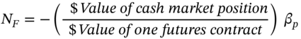
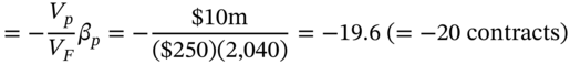
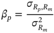
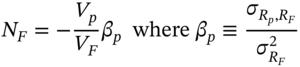
Instead of working out the number of futures contracts you need when you consider a particular fall (e.g. 10%) in the market index, perhaps the ‘best’ formula to use (known as the minimum variance hedge ratio) is to calculate the number of futures contracts using:
where, ![]() ,
, ![]() and
and ![]() .
. ![]() is the ‘dollar value of one futures contract’ and is also sometimes referred to as the ‘invoice price’ or ‘contract price’ of the stock index futures. But note that it is a purely notional amount, since this money is not paid at inception of the futures contract (only a small margin payment is made).
is the ‘dollar value of one futures contract’ and is also sometimes referred to as the ‘invoice price’ or ‘contract price’ of the stock index futures. But note that it is a purely notional amount, since this money is not paid at inception of the futures contract (only a small margin payment is made).
What is important in hedging is that the change in the futures index is (approximately) matched by the change in the (underlying) S&P 500 stock index. The (arbitrary) use of $250 simply converts a 1 point change in the futures index to a dollar amount.6
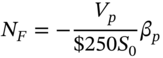
The negative sign means Ms Midas needs to short 20 contracts. The above formula gives an answer very close to our ‘simple’ method described above. But it also has the advantage that you can just ‘plug in’ the known value for the (index) futures, ![]() , currently quoted in Chicago (or on your trading screen). A slight variant to Equation (5.7) is to use the dollar value of the S&P 500 stock index
, currently quoted in Chicago (or on your trading screen). A slight variant to Equation (5.7) is to use the dollar value of the S&P 500 stock index ![]() in the denominator, where
in the denominator, where ![]() is the current level of the S&P 500 stock index, then:
is the current level of the S&P 500 stock index, then:
Because ![]() and
and ![]() do not differ greatly, the above two formulas usually give similar answers for
do not differ greatly, the above two formulas usually give similar answers for ![]() . Notice that in the above we used stock index futures contracts to hedge a portfolio of stocks – and this is usually the case in practice. But you might also wish to hedge your holdings of individual stocks (e.g. Microsoft). Here you have an alternative which is to use a futures contract on Microsoft stock, itself. The above formula still applies but of course here the futures contract on Microsoft has a beta of unity (with respect to Microsoft's stock return). You can also use the above formulas (with slight modifications) to set up a hedge position for oil, wheat, foreign exchange, etc. (see Appendix 5).
. Notice that in the above we used stock index futures contracts to hedge a portfolio of stocks – and this is usually the case in practice. But you might also wish to hedge your holdings of individual stocks (e.g. Microsoft). Here you have an alternative which is to use a futures contract on Microsoft stock, itself. The above formula still applies but of course here the futures contract on Microsoft has a beta of unity (with respect to Microsoft's stock return). You can also use the above formulas (with slight modifications) to set up a hedge position for oil, wheat, foreign exchange, etc. (see Appendix 5).
5.3.2 Hedging in Practice
Let us now consider a slightly more complex hedging example using SIF, where we explicitly calculate futures prices, use the CAPM equation to work out the expected return on the stock portfolio and where the stocks in the portfolio earn dividends. It is 28 December and Ms Midas holds a $10m portfolio of stocks and she wishes to hedge over the next 3 months (to 28 March). She uses the June-futures index to hedge.
28 December, Ms Midas Portfolio (Hedge period = 3 months)

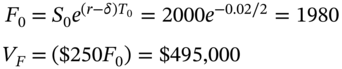
28 December: Stock Index Futures
Maturity of June-forward contract = 6 months (i.e. ![]() year)
year)
Dividend yield on market index ![]() (continuously compounded)
(continuously compounded)
28 March (3 months later)
Assume the S&P 500 has fallen by 10% to ![]() and Ms Midas closes out her June-futures contracts, which now have 3 months to maturity
and Ms Midas closes out her June-futures contracts, which now have 3 months to maturity ![]() :
:
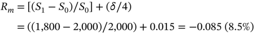
The percentage return on the market portfolio (S&P 500)![]() is the capital loss plus the dividend yield (over 3 months):
is the capital loss plus the dividend yield (over 3 months):
The expected return on your stock portfolio over 3 months (using the CAPM)7:
Expected value of the stock portfolio after 3 months = $10m (1 – 0.1325) = $8.675 m

Percentage change in hedged position (over 3 months) = ($10.0925m/$10m – 1) = 0.925%.
The hedged portfolio has gained $92,500 (0.925% of $10m) in value. Had Ms Midas not hedged she would have lost about 13.25% on her stock portfolio.
The risks in the hedge are:
- beta of the stock portfolio may be estimated incorrectly or it may change over the hedge period.
- The stock portfolio is not well diversified so that some specific risk is present – hence the return on the stock portfolio will not be correctly measured by its beta and the market return.8
- the risk-free rate and the dividend yield – the sources of basis risk – may change over the hedge period (which will alter the correlation between F and S).
The first point is perhaps the most serious and may arise if beta is really time varying but the regression analysis assumes a constant value for beta, estimated using a long data period. The variability in beta can be analysed using recursive regressions – that is, to re-estimate beta as you add more data or you can simply estimate beta over different sample periods, to see how variable its empirical value appears to be. There are also methods for forecasting time varying parameters like beta (e.g. using the Kalman filter). Alternatively, note that a time varying beta can also be directly calculated by using direct estimates of variances and covariances:
The modelling of time varying variances and covariances using ARCH and GARCH models (see Cuthbertson and Nitzsche 2004, 2008) has been rather successful (especially with ‘high frequency’, daily data) and these models can also be used to forecast ![]() over the hedge period using (5.13). There is some evidence that this may improve the hedge outcome compared with using a fixed value for
over the hedge period using (5.13). There is some evidence that this may improve the hedge outcome compared with using a fixed value for ![]() (see, for example, Baillie and Myers 1991). Also note that the hedge ratio given by Equation (5.7) implies that as stock prices change, we should re-calculate
(see, for example, Baillie and Myers 1991). Also note that the hedge ratio given by Equation (5.7) implies that as stock prices change, we should re-calculate ![]() and hence
and hence ![]() periodically. The return on a stock portfolio is:
periodically. The return on a stock portfolio is:
The SIF hedge removes the market risk ![]() , (see Chapter 6) so one source of the hedging error is specific risk
, (see Chapter 6) so one source of the hedging error is specific risk ![]() . The dollar hedging error
. The dollar hedging error ![]() and the variance of the hedging error are:
and the variance of the hedging error are:
It is shown (see Chapter 6) that the variance of the (dollar) hedging error can also be expressed as:
where ![]() is the ‘R-squared’ from the OLS regression (5.14). Equation (5.15c) can be used to calculate the expected error in the hedge.
is the ‘R-squared’ from the OLS regression (5.14). Equation (5.15c) can be used to calculate the expected error in the hedge.
5.4 TAILING THE HEDGE
There is one other practical issue we should deal with, namely adjusting the hedge to take account of interest paid or received on the margin account. This is called ‘tailing the hedge’. Suppose you hedge with a short futures position. If the futures price rises, your short position will make losses, and you may have to make additional margin payments which will increase the overall cost of your hedge. You could offset this increased cost, if you also held some additional long futures positions which would increase in value, when futures prices increase. Hence, if you are initially short (long) ![]() futures, then tailing the hedge will involve going long (short) some additional futures contracts. The ‘tail’ is always an opposite position to the initial futures position (of
futures, then tailing the hedge will involve going long (short) some additional futures contracts. The ‘tail’ is always an opposite position to the initial futures position (of ![]() futures). One method of calculating this tail adjustment is:
futures). One method of calculating this tail adjustment is:
where ![]() is the number of contracts to tail the hedge,
is the number of contracts to tail the hedge, ![]() = the initial number of futures contracts (see Equation 5.7),
= the initial number of futures contracts (see Equation 5.7), ![]() is the risk-free lending or borrowing rate on variation margin payments (any surplus over the maintenance margin is assumed to remain in the margin account), T = time to maturity of the futures. Suppose initially using Equation (5.7) you require
is the risk-free lending or borrowing rate on variation margin payments (any surplus over the maintenance margin is assumed to remain in the margin account), T = time to maturity of the futures. Suppose initially using Equation (5.7) you require ![]() (short) futures contracts on the S&P 500 and the maturity of the futures is
(short) futures contracts on the S&P 500 and the maturity of the futures is ![]() . If the futures index increases by one point, then the short-futures position will lose value:
. If the futures index increases by one point, then the short-futures position will lose value:
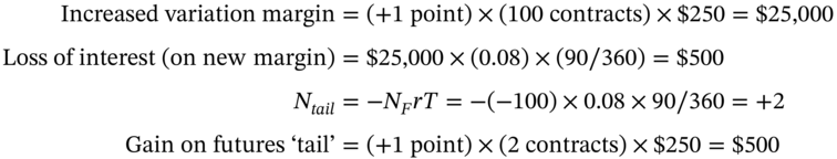
Hence, with ‘the tail’ in place, the additional interest cost of the variation margin is offset by tailing the hedge. In practice, ![]() will vary over the life of the futures and hence tailing the hedge will not produce the perfect result given above. Of course, given the initial
will vary over the life of the futures and hence tailing the hedge will not produce the perfect result given above. Of course, given the initial ![]() contracts and
contracts and ![]() contracts, then the actual initial hedge position taken would have been to short 98 contracts:
contracts, then the actual initial hedge position taken would have been to short 98 contracts:
The value for ![]() , which ‘tails the hedge’ has to be recalculated periodically and the hedged position rebalanced as r and T change.
, which ‘tails the hedge’ has to be recalculated periodically and the hedged position rebalanced as r and T change.
5.5 SUMMARY
- There are a number of different index futures contracts on various stock market indices.
- Index futures prices can be determined using the cost-of-carry approach and violations of this relationship give rise to (risk-free) arbitrage – known as program trading, which today involves high-frequency trading on electronic exchanges, using computer algorithms.
- Stock index futures (SIF) provide a low cost method of hedging an existing diversified equity portfolio or in hedging a future purchase of a diversified portfolio of stocks.
- Hedging using SIF is not perfect, because the changes in the index futures price will not exactly match changes in the stock index (S&P 500) and the portfolio beta is an estimate and may not be accurate over the hedge period. There are also transactions costs in the futures market to consider and potential margin payments.
APPENDIX 5: HEDGE RATIOS
In this appendix we use a common methodology to derive the optimal number of futures contracts required in a variety of practical hedging situations. To calculate the hedge-ratio where the underlying asset to be hedged (e.g. crude oil) is the same as the underlying asset in the futures contract (i.e. futures on crude oil), is straightforward. For example, suppose it is January and you expect to sell 10m barrels of crude oil in 3 months' time in April and you are worried that the oil price in the cash market might fall over the next 3 months. The contract size for one futures on crude oil is for delivery of ![]() barrels, hence to hedge you would short:
barrels, hence to hedge you would short:
Cross Hedge
Now consider the case where the cash market asset you wish to hedge differs from the asset deliverable in the futures contract – this is a cross hedge. To demonstrate a ‘quick method’ of deriving the hedge ratio, assume the airline AirOFly wishes to hedge a future cash market purchase of jet fuel using heating oil futures. (We assume there are no highly liquid futures contracts on jet fuel).9 We have:
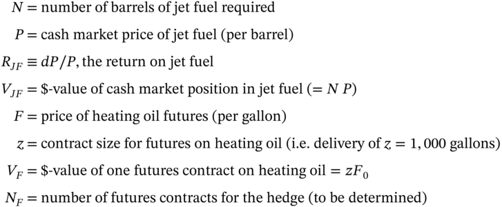
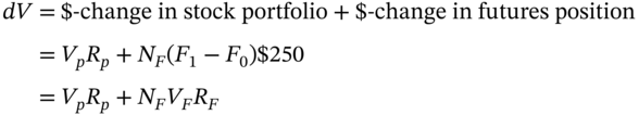
The dollar change in the hedge-portfolio is:
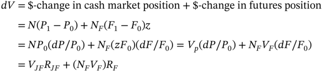
The proportionate change in cash market jet fuel prices (i.e. the return on jet fuel) is ![]() . The return on heating oil futures is defined as
. The return on heating oil futures is defined as ![]() . But
. But ![]() depends on the cash market price of heating oil,
depends on the cash market price of heating oil, ![]() and arbitrage ensures futures and spot prices of heating oil move together. Hence
and arbitrage ensures futures and spot prices of heating oil move together. Hence ![]() where
where ![]() is the percentage change in the spot price of heating oil. We assume that the return on jet fuel and heating oil (spot) prices are linearly related,
is the percentage change in the spot price of heating oil. We assume that the return on jet fuel and heating oil (spot) prices are linearly related, ![]() . A hedge position should involve neither a gain nor a loss so we set
. A hedge position should involve neither a gain nor a loss so we set ![]() and after rearranging:
and after rearranging:
This is the ‘quick method’ of obtaining the optimal hedge ratio.10 It is fine except that the relationship for beta, ![]() will only hold ‘on average’ – so the hedge will not give
will only hold ‘on average’ – so the hedge will not give ![]() exactly – but over a number of hedges the dollar change in value
exactly – but over a number of hedges the dollar change in value ![]() should be small. As we see below, given that prices are stochastic what we are really trying to do in the hedge is to choose that value for
should be small. As we see below, given that prices are stochastic what we are really trying to do in the hedge is to choose that value for ![]() which minimises the variance of
which minimises the variance of ![]() . The correct expression for beta comes from a regression of spot jet fuel returns on the (spot) returns on heating oil:
. The correct expression for beta comes from a regression of spot jet fuel returns on the (spot) returns on heating oil:
Sometimes for hedging over short time periods, absolute rather than percentage changes in prices are used to obtain an estimate of beta, ![]() – but the two methods usually give similar estimates.
– but the two methods usually give similar estimates.
Hedging a Portfolio of Stocks
We can use the above analysis with minor re-definitions to hedge a portfolio of stocks.
Long in the Cash Market
The cash market position consists of n-stocks with ![]() dollars in each stock and a total amount invested of
dollars in each stock and a total amount invested of ![]() dollars. The change in value of the stock portfolio is:
dollars. The change in value of the stock portfolio is:
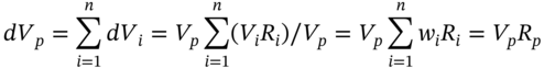
where 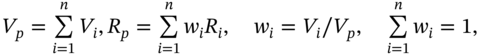
For example, if you hold ![]() in a diversified portfolio of stocks and the return on the portfolio is
in a diversified portfolio of stocks and the return on the portfolio is ![]() over 1 month (say) then your stock portfolio falls in value by $100,000. The change in the dollar value of a hedged portfolio consisting of
over 1 month (say) then your stock portfolio falls in value by $100,000. The change in the dollar value of a hedged portfolio consisting of ![]() dollars held in a stock portfolio and
dollars held in a stock portfolio and ![]() , stock index futures (SIF) is:
, stock index futures (SIF) is:
where ![]() and
and ![]() . We assume that the index futures price
. We assume that the index futures price ![]() and the stock market index (S&P 500) move together (because of arbitrage) so
and the stock market index (S&P 500) move together (because of arbitrage) so ![]() (and
(and ![]() where
where![]() index). If we assume the return on our portfolio of stocks is (exactly) linearly related to the market return,
index). If we assume the return on our portfolio of stocks is (exactly) linearly related to the market return, ![]() and setting
and setting ![]() in (5.A.4) then:
in (5.A.4) then:
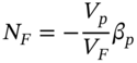
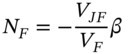
If you are long a portfolio of stocks then ![]() and hence
and hence ![]() and as the betas of nearly all stocks are positive then
and as the betas of nearly all stocks are positive then ![]() . Hence to hedge a long position in a portfolio of stocks, the minus sign in (5.A.5a) indicates that you will short stock index futures.
. Hence to hedge a long position in a portfolio of stocks, the minus sign in (5.A.5a) indicates that you will short stock index futures.
Short-sell in the Cash Market
Let a short-sale of stock-j be represented by a positive (dollar) value ![]() . So a short-sale of say $100 of stock-j implies a positive value for
. So a short-sale of say $100 of stock-j implies a positive value for ![]() . If you short-sell m-stocks then the total value of the short sales is
. If you short-sell m-stocks then the total value of the short sales is 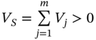 . As we always define the return on a stock as positive (negative) when the price rises (falls) then
 ![]() implies that your cash market short position will increase in value if stock prices fall that is
implies that your cash market short position will increase in value if stock prices fall that is ![]() (and vice-versa). The number of futures contracts to hedge your short position in stocks is then:
(and vice-versa). The number of futures contracts to hedge your short position in stocks is then:
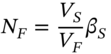
Hence to hedge a short position in stocks, you go long (buy) stock index futures. (This is discussed further in Chapter 6.)
Minimum Variance Hedge Ratio (MVHR)
The correct (and slightly more involved) way to obtain the above expression for ![]() given that prices are stochastic, is to derive the minimum variance hedge ratio MVHR. From (5.A.4):
given that prices are stochastic, is to derive the minimum variance hedge ratio MVHR. From (5.A.4):
where ![]() is the variance of the portfolio return,
is the variance of the portfolio return, ![]() is the covariance between the portfolio return and the index futures return. The value of
is the covariance between the portfolio return and the index futures return. The value of ![]() which minimizes the variance of the hedge portfolio is the solution to
which minimizes the variance of the hedge portfolio is the solution to ![]() , that is:
, that is:
It can be shown that the above expression for ![]() equals the slope coefficient in the OLS regression:
equals the slope coefficient in the OLS regression:
where![]() is the proportionate return on the stock portfolio and
is the proportionate return on the stock portfolio and ![]() is a random error. For SIF we assume (because of arbitrage) that the index futures return
is a random error. For SIF we assume (because of arbitrage) that the index futures return ![]() (in Chicago) equals the return on the S&P 500 market index
(in Chicago) equals the return on the S&P 500 market index![]() (on the NYSE). The ‘market return’ is simply the percentage change in the stock market index
(on the NYSE). The ‘market return’ is simply the percentage change in the stock market index ![]() , so that
, so that ![]() where
where ![]() .
.
A time series regression of portfolio returns ![]() on the market return (S&P 500) gives a direct estimate of
on the market return (S&P 500) gives a direct estimate of ![]() . An alternative is to calculate the portfolio beta from the individual betas of the constituent stocks in the portfolio using
. An alternative is to calculate the portfolio beta from the individual betas of the constituent stocks in the portfolio using ![]() . The individual stock betas11 are obtained from a ‘beta book’ purchased from an investment bank. The
. The individual stock betas11 are obtained from a ‘beta book’ purchased from an investment bank. The ![]() are the proportions held in each stock, where
are the proportions held in each stock, where ![]() is the dollar amount in stock-i and
is the dollar amount in stock-i and ![]() is the total value held in the stock portfolio. Note that replacing
is the total value held in the stock portfolio. Note that replacing ![]() in (5.A.7) by the dollar value of the
in (5.A.7) by the dollar value of the ![]() gives:
gives:
which if ![]() gives approximately the same value for
gives approximately the same value for ![]() as (5.A.7).
as (5.A.7).
EXERCISES
Question 1
You own a stock. A perfect (futures) hedge locks in the current spot price of the stock, after you close out your futures position at some later date (before the maturity of the futures). True or false?
Question 2
In January an investor has a $1.2m long position in a share. The beta of the share is 1.1. The investor intends to close out her position in the share around mid-March and wants to hedge the price-risk using futures. The March Mini S&P 500 future is currently trading at 1,450 (for delivery of $50 times the index). Outline the investor's hedging strategy.
Question 3
You are a US resident. It is 30 January and you plan to purchase a $10m portfolio of around 30 US stocks in 6 months' time with a portfolio beta of 0.5. You are worried about a rise in prices over the next 6 months. The S&P 500 index futures is currently at 1,000.
How could you hedge your future purchases using stock index futures? Would you take a long or short futures hedge?
Question 4
It is 8 November and the stock market index is ![]() . The dividend yield is 3% p.a. and the risk free rate
. The dividend yield is 3% p.a. and the risk free rate ![]() p.a. (both continuously compounded). The December index-futures contract which expires in 40 days (at
p.a. (both continuously compounded). The December index-futures contract which expires in 40 days (at ![]() ) has a quoted price of
) has a quoted price of ![]() . The contract multiple for the index-futures contract is
. The contract multiple for the index-futures contract is ![]() .
.
- Calculate the fair (no-arbitrage) price of the December index-futures.
- Work out an arbitrage strategy with your maximum allowed credit line from the bank of
 .
. - Calculate the risk-free profits, if the stock market index on 18 December (i.e. at maturity of the index futures contract) is
 .
.Assume any stocks you buy or sell ‘mimic’ the movement in the stock market index, that is your stock portfolio has a ‘beta’ of unity.
Question 5
You are the manager of a pension fund with $50m in a diversified portfolio of stocks. You think the stock market over the next 6 months will be more volatile than normal so the potential for losses (and gains) are more extreme – but you believe the stock market will return to ‘normal’ after that. You want to hedge your stock position over the next 6 months and then return to your initial unhedged stock portfolio.
What are the relative merits of selling the stocks and moving into risk-free assets (e.g. T-bills) over the next 6 months, versus using futures contracts to hedge your portfolio?
Question 6
What is the minimum variance hedge ratio, when hedging a portfolio of stocks? Derive the optimal number of futures contracts in the hedge.
Question 7
Suppose you hold a diversified portfolio of stocks with a market value of $10m and a beta of unity. A futures contract on the S&P 500 has 3 months to maturity. Each index point on the futures contract is worth $250. The current interest rate is ![]() (simple rate) and the current value of the S&P 500 stock index is
(simple rate) and the current value of the S&P 500 stock index is ![]() .
.
- Show that the (no arbitrage) ‘fair’ futures price
 (use simple, not compound interest). You want to hedge your $10m stock portfolio over the next month, using stock index futures.
 - How many futures contracts are required to hedge your portfolio of stocks?
- What is the outcome of your hedged position if in 1 month's time the S&P 500 has fallen by 8% and the futures index stands at F1 = 1315.1? Compare the hedged and unhedged positions.
- How do we know that the futures index will be
 (in 1 month's time) after the fall in the S&P 500? Briefly comment on the relationship between the change in the futures and stock indices.
NOTES
- 1 Without the hedge then after 3 months her portfolio could be worth much more or much less – but she does not know in advance which outcome will occur.
- 2 Since 2007, LIFFE is part of NYSE-Euronext.
- 3 To simplify the exposition, we use index points and do not convert to dollars using the value of an index point of $250 – the latter complexity is introduced later in the chapter.
- 4 The futures prices are calculated using
 and
and  , where on 28 December the June-futures has
  years to maturity and on 28 March the June-futures has
  years to maturity. The risk-free rate is
  p.a. and remains constant.
 - 5 More accurately, on average, a sequence of hedges earns a return equal to the risk-free rate – see below.
- 6 This ‘$250’ can be any dollar amount and the formula in (5.8) will ensure the correct number of futures contracts needed for the hedge. Try using ‘$500’ in place of ‘$250’ and you will get a different value for
 but the same outcome, when the futures are closed out.
 - 7 Here, for simplicity, we use the continuously compounded interest rate of 4% p.a., or 1% over 3 months in the CAPM equation. When interest rates are low it makes little difference whether you use the full CAPM equation or the simplified approximation
 .
. - 8 This is because the equation
 really represents the expected return on the stock portfolio. The actual return on the stock portfolio over the hedge period is
  where
where  represents ‘portfolio specific risk’ – and the latter is relatively small but not zero, even in a well-diversified (unhedged) stock portfolio.
 - 9 On the CME there are some traded jet fuel futures, for example Gulf Coast Jet Fuel futures but these are not as heavily traded as heating oil futures.
- 10 You get the same result if you use calculus (which is valid for small changes in the variables). The value of the hedge portfolio is
 . Hence differentiating,
  .
. - 11 These individual betas for each stock-i are obtained from a regression of the excess return on stock-i on the excess market return:
 . Often adjustments are made to the ‘raw estimate’ of beta, for example, using Bayesian shrinkage techniques, where the actual stock beta used is a weighted average of the OLS regression beta and the ‘market return beta’ of 1.