Aims

• To outline the main types of energy and weather derivatives.
• To show how energy derivatives are used for speculation and hedging ‘price risk’.
• To show how weather derivatives are used to hedge ‘volume risk’ of energy producers and users.
• To discuss the use of catastrophe bonds.

There are large oil reserves in a number of countries around the globe, most noticeably the Organisation of the Petroleum Exporting Countries (e.g. the Middle East, Venezuela, Nigeria, etc.) and Russia, who together control about 60% of the world's oil reserves. Russia also has huge natural gas reserves.

Energy prices such as oil and natural gas are highly volatile. This means that large energy suppliers (e.g. in oil exploration and refineries such as BP, Shell, Exxon Mobile) and users of energy (e.g. airlines, transport, and manufacturing companies) face considerable uncertainty about the price they will receive or pay for energy in the future. To mitigate such price risk, consumers and producers can use either over-the-counter (OTC) or exchange traded energy contracts such as forwards, futures, options, and swaps. These ‘commodity derivatives’ are widely used in the energy sector – some are cash settled and some involve physical delivery of the underlying commodity. Electricity is a little different to oil and natural gas since it cannot be stored but its price can also vary tremendously on an hourly basis and derivatives contracts on electricity are also available.

The weather, in the form of abnormally high or low temperatures affects many industries. These include firms who have substantial heating costs in winter or costs of air conditioning in summer, the leisure sector (hotels, ski resorts) and the agricultural sector (e.g. crop growers, vineyards, and orange growers). Abnormal variations in temperature can affect the volume of output produced by these industries which in turn affects their profits. However, derivative contracts based on ‘temperature’ can be used to mitigate these risks due to unforeseen ‘volume effects’.

There are also weather derivatives based on the number of frost days in a month or the depth of snowfall at particular locations. Because the revenues and costs of various industries (e.g. flower growers, municipal authorities, and not least, ski resorts) are affected by frost and snowfall, weather derivatives can be used to mitigate the impact of abnormal levels of snow and frost-days, on the output of these sectors.

In life there is always the possibility of an unusually large natural catastrophe even though this may have a relatively low probability of occurrence – for example, very severe hurricanes, floods and earthquakes. Insurance claims against such events could cause a specific insurance company to go into liquidation, so there is a need to spread such risks across many participants – so called catastrophe (CAT) bonds are one way of doing this.

In this chapter we examine how derivatives are used to hedge (or insure) against price volatility found in spot energy markets and how weather derivatives are used to mitigate changes in profits which result from changes in the volume of output (e.g. in agriculture, energy supply and the hotel and leisure sectors), caused by abnormal changes in the weather.

32.1 ENERGY CONTRACTS

We will not give an exhaustive account of energy derivatives but instead concentrate on the main features of these contracts, so you get a flavour of what is on offer. There has been an active OTC and exchange-traded market in oil products since the early 1980s. OTC forward contracts set a known fixed price today, for future delivery at specific delivery points. Futures and options contracts are traded on crude oil and its refined products, gasoline, heating oil, and jet fuel. The key exchanges trading these contracts are the New York Mercantile Exchange, (NYMEX), the Chicago Mercantile Exchange (CME) and the International Commodities Exchange (ICE) in London. Traded options contracts are usually written on the futures price rather than the cash market (spot) price and are therefore ‘futures options’ – but we largely ignore this nuance in this chapter.

One crude oil futures contract is for delivery of 1,000 barrels, while one jet fuel, heating oil or gasoline futures contract is for delivery of 42,000 gallons (equivalent to 1,000 barrels). Some contracts require physical delivery (e.g. light sweet crude oil futures on NYMEX) while others must be cash settled (e.g. Brent crude oil futures on ICE, Gulf Coast Jet Fuel on CME) and do not allow delivery.

It is only recently that futures and option contracts on jet fuel have been introduced on CME. These trade Sunday to Friday 6 p.m.–5 p.m. on the Globex platform, with a 60-minute break each day (beginning at 5 p.m.). Monthly contracts are available for 36 consecutive months and one contract is for delivery of 42,000 gallons. These are ‘average price’ futures contracts as the floating price for each futures contract month is the arithmetic average of the daily high and low (‘Platts’ jet fuel) spot prices averaged over each business day in the month. Gulf Coast Jet Fuel options are European and also have a payoff which depends on the average price over the month – so they are Asian average price options.

There is also the possibility of avoiding delivery arrangements set by the exchange and instead using ‘exchange of futures for physicals’ (EFP) arrangements, prior to maturity. This is simply a bilateral agreement about location and price, for delivery between the party with the long futures position and the party with (an equal contract size) short position. The futures exchange (clearing house) must be notified of the EFP arrangement and the futures positions for both parties are then terminated. EFP might be used when the long wants delivery at a specific location that is different from that stipulated in the futures contract – if it cost more in transportation and insurance costs to deliver to the long's desired location then the holder of the long futures position will pay an additional cash amount to the trader holding a short position.

There are also OTC and exchange traded contracts on natural gas. Delivery is ‘through the pipe’ at a specific geographical location, at a specific uniform rate through the month. The seller of natural gas (e.g. short futures position) is responsible for delivery at a specific delivery point, for example at the Henry Hub gas interconnector (in Louisiana) or at Zeebrugge (in Belgium) – a key European hub. The supplier of gas might be a separate company to the producer of the gas – particularly in deregulated gas markets such as the USA and UK. NYMEX and ICE trade futures (and options) contracts which (if not closed out) require physical delivery of 10,000 million British thermal units (mbtu) of natural gas. Of course, if you go to delivery and you need your gas in Boston, then you had better make sure you have purchased capacity in the pipe between the Louisiana delivery hub and Boston – because the pipe might be full! Options and swaps on natural gas are also available in the OTC market.

The electricity market is a bit different to oil and gas, as electricity cannot be stored. (Technically you can store it in a battery but this might require a very large battery.) In the US and UK electricity is produced primarily in gas-fired, coal-fired, and nuclear plants. The latter provide the base load and extra demand is met by gas and coal-fired plants (and some by wind turbines and solar). The transmission of electricity is costly and there are also transmission losses to consider, over long distances. So, electricity in the US is provided first to a specific region and any excess can then be sold in the wholesale market. Spikes in electricity consumption can be triggered by abnormally high temperatures in summer (particularly in the US where air conditioning is widely used) or abnormally low temperatures in winter. So there is considerable volatility in electricity prices on a daily basis.

There are active markets in the US and UK in OTC forwards, options and swaps on electricity prices and NYMEX and ICE trade a futures contract on the price of electricity. The contracts allow one party to receive a specified number of megawatt hours, at a specified price and location, during a particular month. For example, this could be a contract, for Monday to Friday only during off-peak hours (11 p.m. to 7 a.m.) within a specified month. There is also a contract for peak hours (7 a.m. to 11 p.m.) from Monday to Friday or a contract for delivery over 24 hours, for 7 days.

With an option contract on electricity you have precisely that – an option to take delivery at the strike price or not. If the contract is for daily exercise, then with one day's notice you can choose whether you want to take delivery of electricity at a price , for the next day. For an option with monthly exercise, you make a decision at the beginning of the month whether you will take delivery of electricity each day at the strike price .

In electricity and natural gas derivatives markets you can also be a ‘swinger’. You can purchase a swing option (also called a take-and-pay option). For an ‘electric swinger’, the option holder sets a maximum and minimum amount of power she will take on each day during a specific month and a maximum and minimum over the whole month. Each megawatt taken is at the strike price, . You can then ‘swing’ the amount of power you choose to take each day (within the bounds set), although there is also usually a limit on the number of days on which you can change your rate of daily consumption.

At this point it is also worth mentioning another market which is likely to be of increasing importance in the future – carbon trading. This is a market where permits can be purchased by firms wanting to increase their output of greenhouse gases. The supply of permits is provided by firms who have been given an allocation of permits which exceed their output of greenhouse gases (see Finance Blog 32.1).

32.2 HEDGING WITH ENERGY FUTURES

32.2.1 Running an Airline

Suppose you own a medium-size US airline ‘EasyFly’ and your marketing manager has told you the ticket prices you will be charging on all your routes, based on maintaining your competitive position in the market. If jet fuel remains at its current level it is estimated that EasyFly will make a handsome profit over the next 3 years. But that is a big ‘if’, in today's volatile oil market. If EasyFly does nothing and jet fuel remains at its current level (or falls) you will be a happy CEO and your shareholders will be smiling too. But if jet fuel rises in price, then despite all your efforts on the technical side (reliability, customer service, maintenance, staff costs, etc.) EasyFly will end up with lower profits and you may lose your job as CEO.

Here we demonstrate the use of a cross hedge so we assume EasyFly hedges some or all of its projected jet fuel costs, using heating oil (HO) futures contracts (traded on NYMEX) rather than futures on jet fuel prices. Since EasyFly fears a rise in spot jet fuel prices in the future it should go long (buy) heating oil futures today. If spot jet fuel prices do rise over the next year, so will the futures price on heating oil and EasyFly can close out its HO-futures contracts on NYMEX at a profit – the latter offsets the higher cost of EasyFly's spot jet fuel.

What practical issues are involved? EasyFly has to decide what quantity Q (gallons) of fuel to hedge and then calculate the appropriate number of futures contracts for each month:

(32.1)

Beta , is the slope of a (OLS) regression with the change in the spot price of jet fuel as the dependent variable and the change in the futures price of heating oil as the independent variable. In practice either of the following equations are used to estimate beta: , or . Since heating oil and jet fuel prices correspond to different ‘commodities’ this is a ‘cross hedge’.

As you have to estimate the relationship between these two price changes, your hedge will be less than perfect – this is basis risk. However, over short horizons of say 1 year, the correlation coefficient (and ‘beta’) between changes in heating oil and jet fuel prices is quite high (the beta is around 0.9) and is reasonably stable over time – so, on average your hedge will work.

But basis risk is also affected by changes in the convenience yield, that is, the premium that holders of heating oil place on having the ‘physical’ heating oil available to satisfy their normal customers – this can cause a divergence between changes in the spot and futures prices at particular periods and could lead to an increase in the hedging error.

Suppose in January EasyFly decides to hedge 2 million gallons of jet fuel for each of the months of April, May, and June. The contract size for heating oil futures is 42,000 gallons (equivalent to 1,000 barrels) hence the number of futures contracts for each month of the hedge is 47.6 (48). So in January EasyFly goes long 48-April, 48-May, and 48-June contracts – taken together this is referred to as a strip hedge.

If EasyFly closes out each contract just before its maturity date this will provide a reasonably good hedge – any gains/losses on the futures contracts will closely offset any increased/lower costs of the spot jet fuel in April, May, and June. Effectively, EasyFly ‘locks in’ a known average purchase price for jet fuel, approximately given by the average of the current quoted futures prices in January for the April, May, and June futures contracts. EasyFly will not take delivery in the futures contracts because it requires physical jet fuel (at various airports around the country) and the futures contract it has used delivers heating oil to New York Harbour – also, planes don't fly well on heating oil!

32.2.3 Collar

Go back to the example of EasyFly that capped the price of its future purchases of fuel by buying a call with a strike, . But buying the call may be expensive. Today, on 15 January EasyFly could offset some of the cost of the call premium C, by selling a put (with strike price ) and receiving the put premium P. If EasyFly, who will purchase fuel in the future, undertakes a ‘buy call-sell put’ position then this is known as a collar (and if the call and put premia exactly offset each other it is known as a zero-cost collar). We know what happens if fuel prices rise, the call sets the maximum effective cost of fuel purchases at . But what happens if fuel prices fall substantially?

If the airline had not sold the put, it would directly benefit from very low spot prices . But if EasyFly has sold a put and if on 15 April, it will have to pay out to the holder (buyer) of the put. If , the effective cost of fuel for EasyFly is equal to the spot price of fuel plus Easyfly's cash payout on the put = . Hence if , the minimum effective cost of the fuel by the airline will be $1.6 per gallon (even if spot fuel prices are below $1.6). So if EasyFly has to purchase airline fuel in the future and it also undertakes a collar trade, it will cap its effective cost at an upper level , but also set a floor level it will pay for fuel of . (Note that for the above to work as described, .)

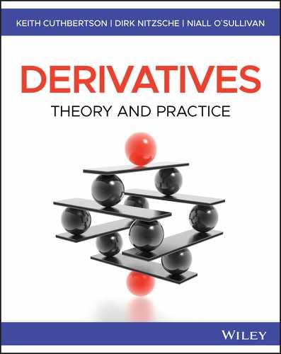
The effective cost (ignoring the cost of the call and the put) of the jet fuel to EasyFly is given in Figure 32.1. If the spot price turns out to be between and , say then neither of the options is in-the-money and EasyFly purchases fuel at the spot price of $1.8.

The key outcome of a collar trade for EasyFly is that it sets a maximum and minimum price for fuel paid by the airline.

32.3 ENERGY SWAPS

We have already discussed interest rate and currency swaps in previous chapters. Now we examine how the energy sector might use swaps to offset any price risks they face. Suppose in January a company such as Centrica in the UK agrees to supply natural gas (NG) to a large industrial customer-ABC (e.g. manufacturing firm) at a fixed price , every month for a 6-month period beginning on 1 January. Centrica decides it will buy the gas in the spot market at whatever price it has to pay at the time of purchase (i.e. it pays a ‘floating price’, to the gas producer who supplies the gas via the European hub at Zeebrugge in Belgium) – Figure 32.2.

Clearly, if the spot price of gas rises, the profit margin of Centrica will be squeezed (and it may even be committed to supplying the gas at a loss if the spot price in Zeebrugge rises above . How can it offset this price risk without renegotiating any of its existing contracts with its customers? It can undertake a receive-fixed, pay-floating swap from a swap dealer where is the floating price used and is the agreed fixed price (see the left-hand side of Figure 32.2). is the swap rate. If the spot price of NG in Zeebrugge at the end of any month is higher than then Centrica receives a cash payment of from the swap dealer. If Centrica buys gas in the cash market at , then the effective cost of Centrica's gas purchases is:

(32.2)

The net result is that Centrica receives from its industrial customers and pays the swap dealer . As long as is greater than , Centrica will have locked in a fixed profit margin of on 1 January, on each unit of NG supplied over the next 6 months.

There are other important elements to the swap deal. There will be a notional quantity of NG in the swap, for example this might be million mbtu per day and the ‘tenor’ of the swap could be every month from January to June. The swap payments to Centrica would then be:

(32.3)

where ‘days’ = number of days in the month. The swap contract may be cash settled each month and it is then a ‘contract for differences’ as only the net cash payment is made by one of the parties to the swap contract. If, in any month:

, then Centrica receives cash from the swap dealer.

, then Centrica pays cash to the swap dealer.

The floating index will have to be decided upon and this spot price often goes under rather strange names; for example, for the Centrica deal it might be the ‘front of month inside FERC’ index. In fact, the floating payment you receive from the swap dealer is based on the ‘front of month’ (FOM) price but Centrica might buy its NG at spot prices throughout the month, so there is some residual price risk remaining.

32.3.1 Pricing the Swap

The fixed price for NG (say) quoted in the swap is the ‘swap rate’ and will vary depending on the maturity of the swap deal – so different swap rates will be quoted for 1-year, 2-year, … etc. swaps. Broadly speaking, the swap rate X is an average of the forward prices for NG over the life of the swap – in terms of jargon, ‘the swap is priced off the forward curve’ (i.e. forward prices of NG at different maturities – see Figure 32.3).

The floating cash flows in the swap depend on future spot prices and our best guess (at ) of these prices are the current quoted forward prices, . The notional volume in the swap contract can be different in different months. The risk-free discount rate is – using continuously compounded rates. The swap is priced at inception so that it has zero value to both parties:

The swap must have zero expected value at inception, so the fixed swap rate quoted today is:

(32.4)

Hence the swap rate is determined by a (complex weighted) average of the forward prices of NG and current spot yields, over the life of the swap.

An OTC swap of the above type can be tailor-made by the swap dealer to suit Centrica. It can begin immediately or can have a delayed start (i.e. ‘forward swap’) or it can be made to apply only to specific months when Centrica feels the spot price for NG is likely to be abnormally high. The notional quantity in the swap (e.g. 1 million mbtu of NG per day), can be pre-set at different levels on particular days within a month. Alternatively, the notional quantity can be a fixed daily amount within any one month but with different daily levels applying for each separate month. These would then be referred to as ‘roller coaster swaps’. With a swap, Centrica effectively locks in the effective price it pays for NG, over several months in the future, regardless of whether the spot price for NG in Zeebrugge turns out to be high or low.

Suppose Centrica is happy to receive from the swap dealer when spot prices turn out to be high (and hence has an effective cost of buying NG of ). But when the floating price of NG is less than the fixed price in the swap, Centrica only wants to pay the swap dealer 60% of . For example, if and then the effective cost of buying NG would be , whereas with a plain vanilla swap the effective cost would have been . So the ‘60% swap deal’ allows Centrica to pay less when prices are low and hence participate in some of the benefit of low prices – not surprisingly this is known as a participation swap.

You may have noticed in Figure 32.2 that the swap dealer has taken on risk, since she is paying to Centrica each month and receiving -fixed from Centrica – so if NG prices rise in the future the swap dealer will experience losses. How does the swap dealer deal with this problem? Well, she may be lucky and find an offsetting deal with another party who wants to pay the swap dealer a floating price (with the same maturity and tenor as the original swap with Centrica). This may happen automatically or the swap dealer can shade her price quotes to encourage such swaps. But let us assume (realistically) that even after these offsetting swaps she still ends up as a net payer at a floating price.

We know that the swap dealer fears a rise in . But if there is a futures contract where the underlying asset is the spot price of NG, she can go long (an appropriate number of) futures contracts. Then if increases in the future she can close out the futures at a profit and use this cash inflow to offset the higher floating payment in her swap deal. So in actual fact what derivatives markets are very good at providing is ‘risk spreading’ across a wide array of participants in these markets. The price risk is still there, but each party only holds ‘just a bit’ of it – it is an efficient ‘risk sharing’ mechanism. In short, without derivatives markets households' gas bills might be even higher. The nearby blog shows how electricity producers can ‘lock in’ a profit margin on their power generation plant.

32.4 WEATHER DERIVATIVES

Weather derivatives can be used by companies whose output and hence profits are affected by abnormal movements in ‘the weather’. Whereas most futures contracts are used to hedge uncertain future price movements, broadly speaking weather futures are used to hedge uncertainty about the levels of ‘output’ in future periods (e.g. the number of gallons of heating oil you might sell to consumers in future months).

For the moment let's consider ‘temperature’ as the only ‘weather variable’ influencing revenues, costs, and profits (that is, we ignore such weather factors as the number of frost days, or the depth of snowfalls, which clearly affect some firms' output, like ski resorts). Energy producers and consumers are affected by temperature since this influences the amount of energy (heating oil, natural gas, electricity) used for heating in the winter months and (in the USA) the amount used for air conditioning in summer (see Weather Risk Management Association, www.wrma.org). The volume of agricultural production is also influenced by temperature (e.g. orange growers in Florida), as are leisure industries (e.g. hotel and holiday companies) and some manufacturers (e.g. of cold drinks or ice cream).

To keep things simple at this point, assume there are traded futures and options contracts, whose payoff depends on the temperature (at a particular point in time and at a particular geographical location), relative to an (arbitrary) average daily temperature which we take to be 65 °F. Let us also assume these derivatives contracts apply to a particular month (and we assume all months have 30 days).

Hence on 15 January, if on average market participants believe that the average daily temperature in June will be 70 °F then the current value of the June-weather futures contract will be . The average cooling degree day (CDD) is 5 and the expected cumulative CDDs in June are 150 – this is because a higher temperature than 65 °F is likely to lead to more energy use for ‘cooling’, using air conditioning. Traders would say that the June contract is currently trading at 150 CDD. The futures contract multiple (on CME) is $20 (per cumulative-CDD), so the June-futures price (on 15 January) is .

As you are probably aware, one of the main topics of conversation of the average citizen is what the weather might be like over the coming months. So, one can only assume they might sometimes like to gamble on the weather. Clearly this is possible using traded weather futures. On 15 January assume the June weather futures is trading at 70 °F, equivalent to a price of $3,000 but you think the (average) daily temperature in June will be 80 °F. As a ‘weather speculator’ you should buy June-weather futures at $3,000. In June if your guess turns out to be correct, the June-futures contract (you purchased in January) will be priced at around and your profit on closing out will be $6,000. The latter figure is simply the increase in the average daily temperature of , scaled up by the 30 days and the $20 per index point.

In January the quoted price for the June-futures forecasts 150 CDDs for June (i.e. an average daily temperature of 70 °F). Hence if you thought the average temperature in June would be 68 °F then as a speculator you would sell June-futures in January and hope to close out at a lower price in June.

What would an ‘option contract on the weather’ look like? Assume that on 15 January market participants expect the average daily temperature in June at a particular location (e.g. Portland Oregon) will be 70 °F, so cumulative CDDs for June are . A strike ‘price’ of for the June-options contract therefore corresponds to an expected average temperature in June of 70 °F. Let's take speculation first. If on 15 January, you think the average daily temperature in Portland in June will be higher than 70 °F then you might buy an option on CDD with a strike . If the average temperature in June actually turns out to be greater than 70 °F, the option will be in-the-money and can be exercised at a profit. If it is less than 70 °F, you simply lose your option premium.

32.4.2 Contract Details

Now we have sorted out the general principles of speculation and hedging with weather derivatives, let us look at a few of the contractual and institutional details. The first OTC weather derivatives were introduced around 1997 and are based on the number of daily ‘heating degree days’ (HDD) or ‘cooling degree days’ (CDD), defined as:

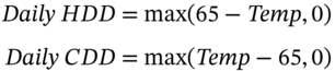
where is the average of the highest and lowest temperature (°F) during the day at a specific location (e.g. at the Chicago O'Hare Airport weather station calculated by the Earth Satellite Corporation). For example if then the daily and the . The monthly HDD and CDD are simply the sum of the daily values. For example, the average daily temperature in Chicago in November is about 50 °F, which is 15 °F below the ‘baseline’ 65 °F set in weather contracts – giving an average daily . Suppose it has been abnormally cold in the Fall in Chicago so the actual out-turn values of daily HDD in November are somewhat lower than average, namely 20, 18, 20, 15, 19, 25, and the other 24 days have . Then the cumulative HDD out-turn for November is 477. Note that when temperatures are low (i.e. well below 65 °F), then HDD is high – a negative correlation. However, CDD increases with temperature (above 65 °F) – a positive correlation.

Lots of ‘bespoke’ weather futures are sold in the OTC market but some plain vanilla contracts are also available with 24-hour electronic trading (e.g. on the CME-Globex trading platform) – both weather futures and European options (on weather futures) are based on the monthly (cumulative) HDD or CDD. These products are also available as seasonal products. The winter season is November to March and the summer season May to September, although April can be added to the summer and October to the winter season, so all months can be covered. You can choose from 2 to 6 months in a seasonal strip contract, so you might choose say 3 months (December, January and March) from the winter season strip, as these may be the months when your (energy) needs are highest but also most volatile and hence may need to be hedged. The CME clearing house guarantees trading on Globex by requiring ‘performance bond’ deposits (i.e. collateral placed in a margin account) at each level in the clearing process – customer to broker, broker to clearing firm, and clearing firm to clearing house.

There are also weather derivatives which have payoffs that depend on the number of frost days in the month or on the depth of snowfall at particular geographical locations. These derivatives work along the same broad principles as weather derivatives based on temperature, as described above. Forwards and futures contracts written on frost days allow firms to protect their profits due to abnormal volume changes in their business, caused by abnormal severe frosts in particular months in particular locations (e.g. wine growers in Napa and Sonoma Valley in California who suffer if grapes are harmed by severe frosts, particularly in spring when the vines are most vulnerable; ditto flower growers in Holland).

The payout from snowfall derivatives is based on the number of inches of snow measured at specific locations at specific times of the day. If there is less or more daily snowfall than average in particular months, the ‘snow derivative's’ payoff at maturity will reflect this outcome. The most obvious case where snow derivatives can be used is by owners of businesses in ski resorts. If there is a lack of snow at particular ski resorts (and sometimes if there is too much snow and risk of avalanches), firms operating in this market can suffer abnormal losses. Also, excessive snowfalls can also severely disrupt the revenues and costs of transport companies, such as road haulage (the trucking business).

Options contracts allow you to purchase insurance. For example, in November a wine grower might buy a call option on ‘frost days’ in March. The call option pays out depending on the number of frost days (above the strike ‘price’ of a fixed level of frost days in the month) and this compensates wine growers for any deterioration in the grape harvest, due to frost. On the other hand, if the number of frost days in March is below the ‘strike rate’ then the call expires out-of-the-money but the grape grower (vigneron) has the benefit of a healthy crop of grapes to make excellent ‘grand cru’ wines (hopefully). The payment of the call premium is the cost of this insurance.

32.5 REINSURANCE AND CAT BONDS

We have seen how weather derivatives can be used to hedge and provide insurance when there are abnormal weather conditions. In general OTC and exchange traded weather derivatives are used to hedge changes in temperature (or frost days or lack or excess of snowfall) which are slightly different from ‘average’. These products are provided in the OTC derivatives market by large banks, specialist energy firms,³ and insurance companies. On the other hand, extreme weather conditions such as hurricanes, earthquakes, and floods are generally dealt with via some form of explicit insurance contract with an insurance company.

Any single insurance company might hold a large number of catastrophe insurance contracts and may therefore be carrying a lot of risk, from low probability but highly costly events. To mitigate some of this risk an insurance company may reinsure say 70% of its risks with other companies, leaving it liable to only 30% of any claim (Lloyds of London is probably the oldest organisation providing such ‘reinsurance’). Alternatively the insurance company can purchase a series of reinsurance contracts for excess cost layers. If the insurance company has $100m exposure to hurricane damage in Florida then it may issue (separate) excess-of-loss reinsurance contracts to cover losses between $40m and $50m, $50m, and $60m etc. Between $40m and $50m of losses, the insurance company receives a dollar-for-dollar payoff from the reinsurer but receives nothing from this particular reinsurance contract if losses are outside this range. Hence, for the first reinsurance contract, the insurance company has the equivalent of a long bull spread – namely, a long call at a strike of $40m and a short call at a strike of $50m.

Reinsurance contracts are very useful but the insurance company can also issue bonds to cover catastrophic (CAT) risks. These have a liquid secondary market and can be sold to many investors thus ‘spreading’ the catastrophic risk more widely. CAT bonds pay a higher than average interest (coupon) but the holders agree to cover the ‘excess-of-loss’ insurance. For example, by issuing $10m principal of CAT bonds an insurance company could cover losses between $40m and $50m by not re-paying some or all of the principal on the CAT bonds, should these losses occur. Alternatively it can make a much larger bond issue, with the covenant that any losses between $40m and $50m will be covered by a reduction in interest payments.

The demand for CAT bonds by investors arises from the fact that they pay higher coupons (or yield to maturity) and the returns on CAT bonds have an almost zero correlation with stock market returns and hence have no systematic risk. In a diversified stock portfolio specific risk will be small but adding CAT bonds can improve the (mean-variance) risk-return trade off in any already well diversified stock portfolio.

32.6 SUMMARY

• Forwards, futures, options, and swap contracts on the price of energy products (oil products, natural gas, electricity) are available OTC and as exchange traded products.
• Energy derivatives can be used to hedge (forwards, futures and swaps) and to provide insurance (options) against future changes in spot energy prices.
• Some contracts are cash settled and others involve delivery – although alternative delivery arrangements from those stipulated in the contract can be separately negotiated and this is known as ‘exchange of futures for physicals’ (EFP).
• Weather derivatives can be used to hedge (or provide insurance) against changes in the volume of energy used by industries whose profits depend on the weather.
• The most actively traded weather derivatives are based on temperature at particular locations at specific times but others depend on the number of frost days or the depth of snowfalls.
• The key exchanges for energy derivatives are the New York Mercantile Exchange (NYMEX), the Chicago Mercantile Exchange (CME) and the International Commodities Exchange (ICE) in London. There is also a very large OTC market.

EXERCISES

Question 1

You will have to purchase 560,000 barrels of (spot) jet fuel in 1 year's time. There is a futures contract available on heating oil which you are going to use to hedge your jet fuel purchases.

Contract size for heating oil is 42,000 barrels. Changes in jet fuel and heating oil prices have a beta of 0.9.

How would you implement the hedge and explain what happens if the spot price of heating oil either increases or decreases over the next year?

What is the effective price of your jet fuel?

Briefly explain why your strategy might not result in a ‘perfect hedge’.

Question 2

It is 22 September and you have agreed to sell 10,000 mbtu of NG at S(fix) = 8.60 $/mbtu to a commercial customer in early January. You do not currently have the NG. You will buy the NG in the cash market at the end of December but you are worried that NG prices will increase between September and the end of December.

On 22 September you decide to hedge your position by using an at-the-money (ATM) option (on NG futures). Assume the options are cash settled. ATM options are available which have a (fixed) strike price K, equal to the current futures price, F₀(Jan) = 8.20 $/mbtu.

Derivatives (22 September)

• The NG-futures for January delivery on NYMEX is $/mbtu
• ATM call costs, (with expiry date of 28 December).
• ATM put costs .
  

  28 December: Price rise

• On 28 December if you decide to exercise your (futures) option you face futures prices and the spot price is also

  28 December: Price fall

• On 28 December if you decide to exercise your option you face futures prices and the spot price is also .

What are the outcomes after using the required futures or options contract in these two cases? Briefly comment.

Question 3

In May, GasCorp has agreed to sell 10,000 mbtu per day of natural gas (NG) at S(fix) = 10.5 $/mbtu to customers in the Boston area for each of the months in the next year from January–June. GasCorp does not currently have the NG. GasCorp will buy the NG in the spot (cash market) in each of the months January–June and hedge these purchases using a NG-swap. The current NG swap rate quoted by CitiGroupEnergy is X = 10.0 $/mbtu.

1. How would GasCorp hedge its January–June purchases using a swap?
2. What is the payoff to GasCorp from the swap each month, if spot-NG prices turn out to be:

   	Spot out-turn, S
   Jan	11.85
   Feb	11.87
   Mar	11.65
   Apr	9.69
   May	9.49
   Jun	9.6

3. What is the ‘effective average price’ GasCorp pays for its NG purchases in each month?
4. How might the swap dealer CitiGroupEnergy hedge its risk in the swap contract?

Question 4

You purchase a large amount of natural gas at the current cash-market price, for heating in the winter months (November to March). In July how might you use futures contracts to hedge your price and volume risk over the winter months? Explain.

Question 5.

Los Angeles: average temperatures in July and August

In February, a large water park in Los Angeles, California owned by the DHockney Corporation called ABiggerSplash, knows that abnormally cool weather (between 65 °F and 70 °F average) over the summer months (July, August) leads to less customers and reduced profits. The ‘normal’ average temperature in July/August is 80 °F. The tick value for weather futures is $100 per °F.

How can the water park mitigate such losses using weather futures?

Does it use futures on heating degree days (HDD) or cooling degree days (CDD)?