CHAPTER 28
The Greeks
Aims
- To show how ‘the Greeks’ (e.g. delta, gamma, rho, vega, and theta) provide useful ‘summary statistics’ for options, which can be used to provide an approximation to the change in the option price.
- To show how the Greeks are used to protect the value of an options portfolio from small changes (delta hedging) and large changes (delta-gamma hedging) in the price of the underlying asset.
- To demonstrate how the Greeks are used to protect the value of an options portfolio from large and small changes in the underlying asset's price, when the latter is also accompanied by (small) changes in volatility – this is ‘gamma-vega-delta’ hedging.
- To demonstrate how to calculate ‘the Greeks’ for the BOPM.
28.1 DIFFERENT GREEKS
The Black–Scholes formula (on a non-dividend paying stock) shows that the option premium varies with ![]() , all of which may change minute by minute. In this chapter we show how the change in price of the option can be represented in terms of a number of ‘summary statistics’ which are generally referred to as ‘the Greeks’. Knowing the numerical values for the various ‘Greeks’ also allows an options trader to set up effective hedge positions for her portfolio of options. As we shall see, the more sources of uncertainty the options trader wants to hedge (stocks, interest rates, volatility) and the smaller the desired hedging error, the more complex the trader's hedging strategy needs to be.
, all of which may change minute by minute. In this chapter we show how the change in price of the option can be represented in terms of a number of ‘summary statistics’ which are generally referred to as ‘the Greeks’. Knowing the numerical values for the various ‘Greeks’ also allows an options trader to set up effective hedge positions for her portfolio of options. As we shall see, the more sources of uncertainty the options trader wants to hedge (stocks, interest rates, volatility) and the smaller the desired hedging error, the more complex the trader's hedging strategy needs to be.
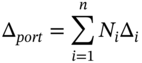
28.1.1 Portfolio Delta
Suppose you have a portfolio of ![]() options consisting of
options consisting of ![]() calls and puts (with different strikes and time to maturity) but on the same underlying stock (e.g. Microsoft). The portfolio delta of the options is defined as:
calls and puts (with different strikes and time to maturity) but on the same underlying stock (e.g. Microsoft). The portfolio delta of the options is defined as:
We take ![]() if you are long (= buy) a call or put and
if you are long (= buy) a call or put and ![]() if you are short (=sell) a call or put.
if you are short (=sell) a call or put.
28.1.2 Gamma
In the following sections we denote the derivatives price as ![]() so our remarks will apply to either call or put options. The gamma of an option is defined as:
so our remarks will apply to either call or put options. The gamma of an option is defined as:
Gamma is the second derivative of the option price with respect to the stock price.1 Gamma is also the change in the option's delta as S changes by a small amount ![]() , hence:
, hence:
Gamma (like delta) takes on different values for different values of ![]() . The relationship between gamma and the stock price (other variables held constant) is roughly ‘bell shaped’ and the maximum value for gamma occurs when the current stock price is close to the strike price – that is, for a ‘near-ATM’ option (Figure 28.1).
. The relationship between gamma and the stock price (other variables held constant) is roughly ‘bell shaped’ and the maximum value for gamma occurs when the current stock price is close to the strike price – that is, for a ‘near-ATM’ option (Figure 28.1).
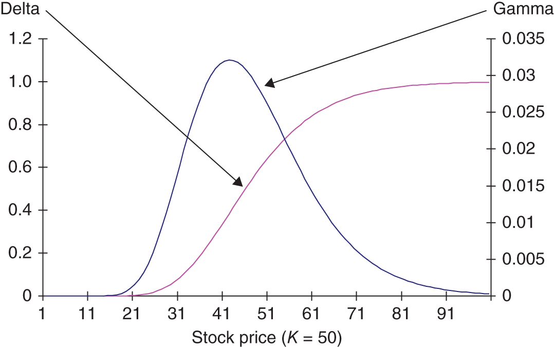
FIGURE 28.1 Delta and gamma – long call
If ![]() and the stock price changes by a small amount (e.g. $1), the slope of the Black–Scholes curve (i.e. the option's delta) will not change by very much, say from 0.5 to 0.53, giving a gamma of 0.03. (However, note that the value of gamma for an ATM option which is also ‘close to maturity’ can be much larger than this – see below.)
and the stock price changes by a small amount (e.g. $1), the slope of the Black–Scholes curve (i.e. the option's delta) will not change by very much, say from 0.5 to 0.53, giving a gamma of 0.03. (However, note that the value of gamma for an ATM option which is also ‘close to maturity’ can be much larger than this – see below.)
Clearly Figure 28.1 shows that when a call is either very ![]() or very
or very ![]() then
then ![]() is small and fairly constant (if the stock price changes by a small amount). This implies that for OTM and ITM options, a delta hedge will work quite well even if you do not rebalance very frequently (e.g. every 5 days), since a small gamma means that delta does not change very much as S changes, from day to day.
is small and fairly constant (if the stock price changes by a small amount). This implies that for OTM and ITM options, a delta hedge will work quite well even if you do not rebalance very frequently (e.g. every 5 days), since a small gamma means that delta does not change very much as S changes, from day to day.
In contrast, for an option that is currently ATM (i.e. ![]() ) then gamma can be relatively large and vary a great deal as S changes (Figure 28.1). A large gamma alerts an options trader who is delta hedging her position, that to remain delta hedged she will probably have to rebalance her portfolio frequently (e.g. twice per day). Alternatively she can ‘eliminate’ the current large value of gamma by ‘gamma hedging’ – see below.
) then gamma can be relatively large and vary a great deal as S changes (Figure 28.1). A large gamma alerts an options trader who is delta hedging her position, that to remain delta hedged she will probably have to rebalance her portfolio frequently (e.g. twice per day). Alternatively she can ‘eliminate’ the current large value of gamma by ‘gamma hedging’ – see below.
The value for gamma is obtained from the Black–Scholes equation for European options (on a stock paying continuous dividends):
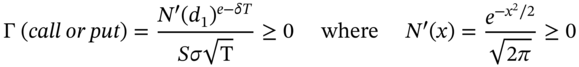
Gamma is positive for either a long call or a long put. Also the gamma for a call is equal to the gamma for a put option (with the same underlying asset, strike price, and time to maturity). To obtain a ‘negative gamma’ you must sell (write) calls or puts.
Gamma is useful when calculating the change in the option price for a large change in the stock price – using gamma is sometimes referred to as a ‘curvature adjustment’. A delta-hedged position does not give protection against large changes in the stock price. This can be seen by noting that the change in the option premium can be approximated by a second-order Taylor series expansion of the option price (with respect to S):
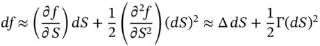
The change in the option price depends on both delta and gamma – as can be seen in Example 28.3.
28.1.3 Portfolio Gamma
The gamma for a portfolio of options (with different strikes and time to maturity but on the same underlying stock) is defined as:
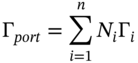
If Ms Smart's options portfolio is delta hedged (i.e. ![]() ) but the gamma of the portfolio of options is large, then the portfolio will not be hedged against ‘large’ changes in the stock price. But if Ms Smart can form a ‘new portfolio’ of stocks and options which makes both the portfolio delta and the portfolio gamma equal to zero, then she is protected from both small and large changes in the stock price – this is ‘delta-gamma’ hedging and is discussed below.
) but the gamma of the portfolio of options is large, then the portfolio will not be hedged against ‘large’ changes in the stock price. But if Ms Smart can form a ‘new portfolio’ of stocks and options which makes both the portfolio delta and the portfolio gamma equal to zero, then she is protected from both small and large changes in the stock price – this is ‘delta-gamma’ hedging and is discussed below.
Note that the ‘gamma of a stock’ is zero – this is because the value of a stock is linear in the stock price. If ![]() then
then ![]() and
and ![]() .
.
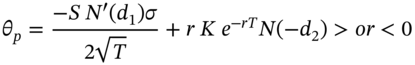
28.1.4 Theta
The change in the option premium due to the passage of time is non-stochastic and is measured by the option's theta (see Appendix 28):
In the Black–Scholes formula ‘time’ is measured in years or fractions of a year and when discussing theta we can take ![]() , so
, so ![]() (years) or we can measure theta per calendar day
(years) or we can measure theta per calendar day ![]() . The option's theta depends on the current stock price, time to maturity, stock volatility, and interest rate.
. The option's theta depends on the current stock price, time to maturity, stock volatility, and interest rate.
Theta is usually negative for most long positions in options – both long calls and long puts lose value as they get closer to maturity (all other variables held constant). Theta is most negative for options that are nearly ATM, so ATM options lose time value rather quickly, day by day. Alternatively, if the current stock price is very low then theta is close to zero (for calls and puts). When the time to maturity is short (e.g. few weeks to maturity) the value of theta for ITM, OTM and especially for ATM options can become relatively large – so these options all lose time value relatively quickly (all other variables held constant).
Note that as ‘time’ is deterministic, the theta of the option is not used in any kind of hedging as there is no uncertainty. Theta is useful as an estimate of the change in value of the option over time. There is another more esoteric use for theta. It can be shown (using the Black–Scholes partial differential equation [PDE], see Chapter 48) that for ![]() in a portfolio of options on a single underlying asset with current price
in a portfolio of options on a single underlying asset with current price ![]() the following holds,
the following holds, ![]() . For a delta-neutral portfolio we have:
. For a delta-neutral portfolio we have:
This shows that for a delta-neutral portfolio, when theta is large and positive the gamma tends to be large and negative – so here theta is also an indication of the gamma-risk in the options portfolio.
28.1.5 Rho
The change in the option price due to a change in ![]() is known as ‘rho’,
is known as ‘rho’, ![]() . For call and put options (for both a dividend paying and non-dividend paying stock):
. For call and put options (for both a dividend paying and non-dividend paying stock):
In the Black–Scholes pricing formula, ![]() is entered as a decimal. Hence, a change in interest rates of 1% is entered as
is entered as a decimal. Hence, a change in interest rates of 1% is entered as ![]() in the formula
in the formula ![]() .
.
Theta and rho are the ‘lesser Greek Gods’ since usually the option premium is not particularly sensitive to either changes in ![]() or changes in the time to maturity.
or changes in the time to maturity.
28.1.6 Vega
The change in the option's premium for a small change in volatility ![]() , is measured by the option's vega
, is measured by the option's vega ![]() :
:

‘Vega’ is not a Greek letter and ‘vega’ is also referred to as lamda, kappa, or sigma, which are Greek letters. The numerical value of vega is the same for a long call or long put (with same strike, time to maturity, and underlying stock) and has a bell shape with respect to the stock price (Figure 28.2). To obtain a ‘negative vega’ you must sell (write) calls or puts.
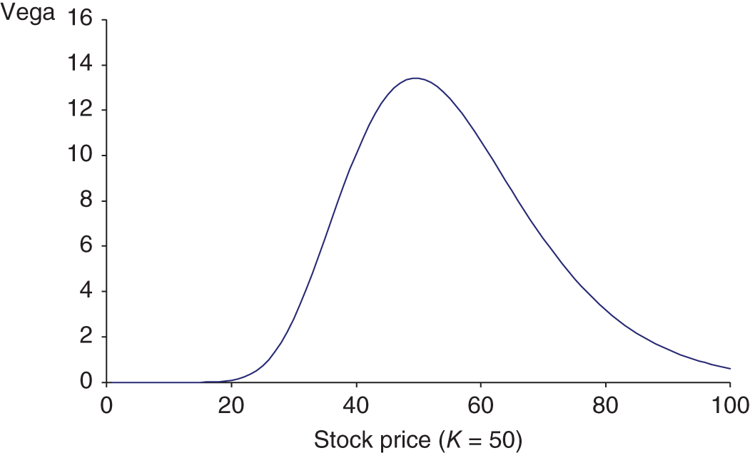
FIGURE 28.2 Vega (long call or put)
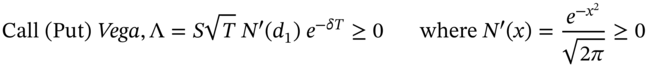
If the vega of an option is large this implies the option price is highly sensitive to small changes in volatility ![]() . For a European option on a stock, the vega is large when the option is close to being at-the-money (i.e.
. For a European option on a stock, the vega is large when the option is close to being at-the-money (i.e. ![]() ) and is zero for options that are well OTM or well ITM (Figure 28.2). The analytic expression for the vega of a European (call or put) option on a stock (or stock index) paying a continuous dividend yield
) and is zero for options that are well OTM or well ITM (Figure 28.2). The analytic expression for the vega of a European (call or put) option on a stock (or stock index) paying a continuous dividend yield ![]() is:
is:
Strictly speaking, using the Black–Scholes vega to hedge against changes in volatility ![]() of the underlying asset is inconsistent – as the Black–Scholes model assumes volatility is constant – but this approach seems to work reasonably well in practice (i.e. even when volatility is stochastic). It should be obvious that the vega of a stock is zero – this is because the value of a stock portfolio does not depend on the stock's volatility (if
of the underlying asset is inconsistent – as the Black–Scholes model assumes volatility is constant – but this approach seems to work reasonably well in practice (i.e. even when volatility is stochastic). It should be obvious that the vega of a stock is zero – this is because the value of a stock portfolio does not depend on the stock's volatility (if ![]() then
then ![]() ).
).
Explicit expressions for ‘the Greeks’ can be obtained if we have a closed-form solution for the option premium. These are given in Appendix 28 for European calls and puts (on a stock that pays a continuous dividend yield), based on the Black–Scholes equation. Using the Greeks enables an options trader to hedge her existing portfolio of options either from small or large changes in the price of the underlying asset, or from changes in volatility and changes in interest rates.
28.1.7 Approximating Option Price Changes
The Greeks also provide a convenient way of finding the approximate change in the option premium ![]() , as all the variables
, as all the variables ![]() change. A Taylor series expansion f the equation for the (Black–Scholes) option price
change. A Taylor series expansion f the equation for the (Black–Scholes) option price ![]() is:
is:
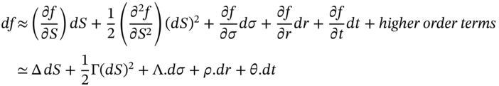
where ![]() = change in the stock price, etc. This is also a useful expression for calculating the approximate change in the option price
= change in the stock price, etc. This is also a useful expression for calculating the approximate change in the option price ![]() , once we have any reasonable way of obtaining estimates of the Greeks (e.g. from an approximate closed-form option pricing equation, from MCS or from the BOPM).
, once we have any reasonable way of obtaining estimates of the Greeks (e.g. from an approximate closed-form option pricing equation, from MCS or from the BOPM).
Note also, that the values for all the Greeks change over time as the values of ![]() and time to maturity
and time to maturity ![]() , change. For example, a portfolio of options which currently has
, change. For example, a portfolio of options which currently has ![]() will not represent a gamma-neutral position some time later because as
will not represent a gamma-neutral position some time later because as ![]() and
and ![]() change over time, so does the option's gamma,
change over time, so does the option's gamma, ![]() .
.
28.2 HEDGING WITH THE GREEKS
28.2.1 Portfolio of Options
Suppose you have a portfolio of ![]() options consisting of
options consisting of ![]() calls and puts (with different strikes and time to maturity) but on the same underlying stock (e.g. Microsoft). The delta, gamma, and vega of the portfolio of options are:
calls and puts (with different strikes and time to maturity) but on the same underlying stock (e.g. Microsoft). The delta, gamma, and vega of the portfolio of options are:

 if long (buy) a call or put
 if short (sell) a call or put
 for long call (from Black–Scholes)
 for long put (from Black–Scholes)
Also, each long stock has a delta of ![]() and a gamma and vega of zero. If you hold (buy) stocks then
and a gamma and vega of zero. If you hold (buy) stocks then ![]() and if you short-sell stocks
and if you short-sell stocks ![]() .
.
28.2.2 Gamma Neutral
The gamma for Microsoft stock (or futures on the stock) are both zero. So, the only way you can change the gamma of an existing options portfolio on several Microsoft calls and puts is to take new positions in some other options on Microsoft. Suppose you already have a portfolio-A, of several calls and puts on Microsoft which have a portfolio delta of ![]() and gamma of
and gamma of ![]() . If you now add a further
. If you now add a further ![]() traded options on Microsoft (with different strike prices and maturity dates) into your existing options portfolio-A, then the gamma of this new portfolio is:
traded options on Microsoft (with different strike prices and maturity dates) into your existing options portfolio-A, then the gamma of this new portfolio is:
Your new portfolio is gamma-neutral ![]() when:
when:
But including ![]() additional options will also alter the overall portfolio's delta. Hence we then buy or sell a number of Microsoft stocks (or futures contracts on Microsoft stock) to make the overall options portfolio delta neutral. An example is given in Example 28.8.
additional options will also alter the overall portfolio's delta. Hence we then buy or sell a number of Microsoft stocks (or futures contracts on Microsoft stock) to make the overall options portfolio delta neutral. An example is given in Example 28.8.
Note that as time passes S, σ, r and T change, hence so do gamma and delta – therefore periodic rebalancing is required to maintain delta-gamma neutrality.
Kurpiel and Roncalli (1998) find that (in a Black–Scholes constant volatility world) when you just delta hedge a call option with rebalancing over either {5, 1, 1/2} days, the percentage hedging error is ![]() 2 whereas with a delta-gamma hedge these figures improve to
2 whereas with a delta-gamma hedge these figures improve to ![]() , which are ‘reasonable’ even when rebalancing takes place only every 5 days.
, which are ‘reasonable’ even when rebalancing takes place only every 5 days.
28.2.3 Vega Neutral
The vega of an existing options portfolio on Microsoft can only be altered by adding another traded option on Microsoft to the existing portfolio. Suppose we initially hold a portfolio of Microsoft stocks with a portfolio vega of ![]() and another option-X on Microsoft is available with a vega
and another option-X on Microsoft is available with a vega ![]() . To obtain a vega-neutral position we require
. To obtain a vega-neutral position we require ![]() options which satisfy:
options which satisfy:
hence
Our new portfolio will not be delta neutral but we know that if we now take a position in Microsoft stocks, we can also achieve delta neutrality. For daily rebalancing in a stochastic volatility world, Kurpiel and Roncalli (2009) report an improvement in hedge performance as we move from purely delta hedging with ![]() , to delta-vega hedging where %HE = 0.135%. However, we still have a potential problem because our delta-vega neutral portfolio may have a non-zero gamma and therefore may not be protected against large changes in the stock price.
, to delta-vega hedging where %HE = 0.135%. However, we still have a potential problem because our delta-vega neutral portfolio may have a non-zero gamma and therefore may not be protected against large changes in the stock price.
28.2.4 Gamma-Vega-Delta Neutral
Agamma-vega-delta neutral position implies that the value of the portfolio is (nearly fully) protected against small or large changes in the stock price and against small changes in the stock's volatility.
Suppose we have a portfolio-A of options on Microsoft which is already vega neutral but has a gamma of ![]() . How can we simultaneously achieve gamma and vega neutrality? At first sight it may seem as if we just include
. How can we simultaneously achieve gamma and vega neutrality? At first sight it may seem as if we just include ![]() new options-X (on Microsoft) to achieve gamma neutrality. However, this is incorrect, as adding the new options-X destroys our initial vega neutrality, because the new
new options-X (on Microsoft) to achieve gamma neutrality. However, this is incorrect, as adding the new options-X destroys our initial vega neutrality, because the new ![]() options themselves have non-zero vegas. To achieve a delta-gamma-vega neutral portfolio we proceed in two steps:
options themselves have non-zero vegas. To achieve a delta-gamma-vega neutral portfolio we proceed in two steps:
- First, we include ‘new’ options on Microsoft (with different strike prices and maturity dates and hence different gammas and vegas) to our original portfolio-A (of Microsoft options), so that we simultaneously achieve gamma-vega neutrality.
- Second, we go long or short Microsoft stocks to make our ‘new’ options portfolio delta neutral – this will not alter our ‘new’ gamma-vega neutrality because stocks have a gamma and a vega of zero.
An example of setting up a ‘delta-gamma-vega’ neutral position is given in Example 28.9.
The value of your ‘final options and stocks’ position consists of your initial portfolio-A of several options on Microsoft (with different strikes and time to maturity) plus our new positions in options-Y and options-Z (on Microsoft) which give gamma-vega neutrality, and finally short-selling Microsoft stocks to achieve delta neutrality. Your new positions in options and stocks means that your ‘final portfolio’ is now hedged against small (delta) and large (gamma) changes in S and also against (small) changes in volatility (vega).
28.2.5 Frequency of Rebalancing
A long call or a long put on a stock (with the same strike price and maturity) have the same positive values for either gamma or vega. Short calls and puts have negative gamma and vega. Although options traders might frequently rebalance their portfolios to maintain delta neutrality, they generally do not rebalance often to maintain gamma and vega neutrality, since it may be difficult to find appropriate ‘offsetting options’ at competitive prices. They therefore adjust their options position to give gamma and vega neutrality only after these ‘Greeks’ become unacceptably large. However, their portfolio of options positions will usually be monitored daily and their potential vulnerability to possible changes in either stock prices or volatility (of stock returns) will be calculated – this is the subject of Chapter 46 on risk measurement.
The options trading desks of many banks mainly write calls and puts for their clients and hence build up negative gamma and negative vega positions, in the normal course of trading. They therefore often step in as buyers of options when these are available at competitive prices, in order to reduce their gamma-vega exposures. Because an option's vega and gamma are large when the options are close to ATM, an options dealer may gamma-vega (and delta) hedge a portfolio of ATM options under these circumstances, even when the options have a considerable time to maturity.
It is also the case that the gamma and vega for ATM options which are close to expiration are exceptionally large and hence the options trader may consider a gamma-vega (and delta) hedge, if she holds options that are both ATM and close to expiration. A trader who initially sells ATM calls and puts and delta hedges her position hopes that the options will become well OTM or ITM, since then the vega and gamma become very small (Figure 28.2) and there may be no need to undertake costly gamma-vega hedging.
A portfolio of futures options (e.g. options on AT&T futures contracts) can be used together with futures contracts (on AT&T stocks) in implementing dynamic delta hedging. An existing portfolio of futures options-A (e.g. on AT&T futures contracts) can be combined with other futures options-B (on AT&T futures contracts, but with different strikes and time to maturity) to simultaneously produce a gamma-neutral and vega-neutral portfolio. Finally, one can use futures contracts (on AT&T) to achieve a portfolio which is gamma-vega-delta neutral.
As we have seen, if you hold a portfolio of options on AT&T stocks then you can gamma-vega-delta hedge using other options (written on AT&T stock) together with the AT&T stocks themselves. However, because the stock price and the futures price move closely together you can also gamma-vega-delta hedge a portfolio of options (on AT&T stocks), using options on futures contracts of AT&T – together with futures contracts on AT&T stocks (to ensure delta neutrality).
28.3 GREEKS AND THE BOPM
Suppose we do not have a closed-form solution like Black-Scholes for option premia but we wish to calculate ‘the Greeks’ for a specific option. We have already seen this in the context of MCS. Now we examine the calculation of the Greeks in the BOPM.
Suppose we construct a lattice for the stock price and a ![]() year option, with
year option, with ![]() steps, so that each time period corresponds to 1 week (
steps, so that each time period corresponds to 1 week (![]() years) and
years) and ![]() and
and ![]() . How can we determine the Greeks so that if we currently hold an option, we can hedge against delta, gamma and vega risk?
. How can we determine the Greeks so that if we currently hold an option, we can hedge against delta, gamma and vega risk?
There are two ways of doing this. The first is to apply the perturbation approach used in the MCS in Chapter 26. Suppose the current stock price is ![]() and we calculate the call premium
and we calculate the call premium ![]() (under RNV) using backward recursion in the binomial tree. To find the option's delta we perturb the initial stock price by a small amount
(under RNV) using backward recursion in the binomial tree. To find the option's delta we perturb the initial stock price by a small amount ![]() , say, so that
, say, so that ![]() is the new initial stock price. We keep everything else unchanged and produce a new tree using
is the new initial stock price. We keep everything else unchanged and produce a new tree using ![]() etc., and calculate the new price for the option
etc., and calculate the new price for the option ![]() . The delta of the option is then calculated as
. The delta of the option is then calculated as ![]() . The option's vega and rho can be calculated in a similar way.
. The option's vega and rho can be calculated in a similar way.
If we want to find the option's gamma (which is the change in the delta as S changes by a small amount) we repeat our calculation for delta but this time using a lattice which starts off with ![]() . Suppose for this lattice we obtain a call premium equal to
. Suppose for this lattice we obtain a call premium equal to ![]() so that our new
so that our new ![]() . Then gamma is given by the change in delta:
. Then gamma is given by the change in delta:
The second way of proceeding is to directly calculate (some of) the Greeks using only the initial tree for ![]() and the tree for the option premium
and the tree for the option premium ![]() . Define the stock price at each node of the tree as
. Define the stock price at each node of the tree as ![]() . We designate i as the number of ‘up’ moves in the lattice (e.g. for UU,
. We designate i as the number of ‘up’ moves in the lattice (e.g. for UU, ![]() ). A ‘down’ move is denoted ‘0’ (which geometrically is represented as a horizontal move – Figure 28.3). Thus at
). A ‘down’ move is denoted ‘0’ (which geometrically is represented as a horizontal move – Figure 28.3). Thus at ![]() ,
, ![]() becomes
becomes ![]() where the ‘1’ represents the number of ‘up’ moves. We also have a similar lattice for the values of the option price
where the ‘1’ represents the number of ‘up’ moves. We also have a similar lattice for the values of the option price ![]() obtained via backward recursion (under RNV). Use of this notation allows the lattice to be represented in computer programs.
obtained via backward recursion (under RNV). Use of this notation allows the lattice to be represented in computer programs.
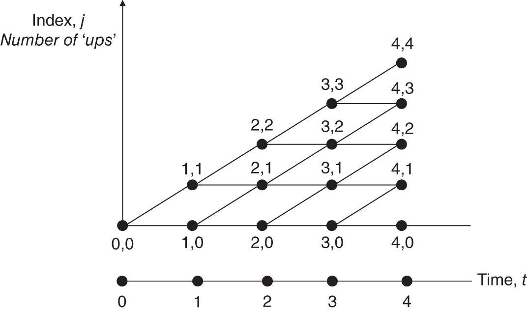
FIGURE 28.3 BOPM lattice
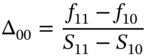
At ![]() we calculate the option's delta at node (0, 0) using:
we calculate the option's delta at node (0, 0) using:
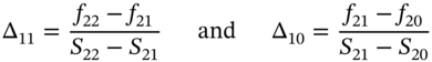
To estimate gamma, note that we have two estimates of ![]() at
at ![]() :
:
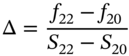
The values of S that correspond to these values of Δ are calculated as follows. The average value of S in the upper and lower parts of the lattice (at ![]() ) are
) are ![]() and
and ![]() . Hence their difference is:
. Hence their difference is:
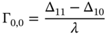
We can now calculate gamma at ![]() , as the change in delta divided by the ‘distance’ between our two measures of delta:
, as the change in delta divided by the ‘distance’ between our two measures of delta:
Even though our estimates of ![]() and
and ![]() require the use of nodes at
require the use of nodes at ![]() and
and ![]() , it is assumed that these represent
, it is assumed that these represent ![]() and
and ![]() at
at ![]() , because the time interval
, because the time interval ![]() in the lattice is small. We can make
in the lattice is small. We can make ![]() as small as we like so we can also obtain estimates of
as small as we like so we can also obtain estimates of ![]() at
at ![]() by approximating the derivatives at other nodes (time periods). For example, using values at
by approximating the derivatives at other nodes (time periods). For example, using values at ![]() an estimate of
an estimate of ![]() is:
is:
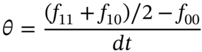
An estimate of the option's theta ![]() (i.e.
(i.e. ![]() held constant) is easily obtained by interpolating between the first two nodes at
held constant) is easily obtained by interpolating between the first two nodes at ![]() . The average value of the option at
. The average value of the option at ![]() is
is ![]() and hence an estimate of
and hence an estimate of ![]() is3:
is3:
An estimate of vega requires two trees as in any single tree, ![]() is constant and
is constant and ![]() and
and ![]() are constant. Hence we must use the perturbation approach. We choose a new value for sigma
are constant. Hence we must use the perturbation approach. We choose a new value for sigma ![]() (where
(where ![]() is small) and calculate new values for U and D and hence a ‘new tree’ for the stock price. We keep
is small) and calculate new values for U and D and hence a ‘new tree’ for the stock price. We keep ![]() ,
, ![]() ,
, ![]() and
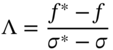
and ![]() unchanged and calculate the ‘new’ option price using backward recursion on the new tree. If the new option price is
unchanged and calculate the ‘new’ option price using backward recursion on the new tree. If the new option price is ![]() , the option's vega is:
, the option's vega is:
The option's rho can be calculated in a similar way to vega by changing the risk-free rate by a small amount (and keeping dt, n, U, D the same as in the original tree) which gives ![]() .
.
28.4 SUMMARY
- Delta hedging one written (sold) call, requires a long position in
 stocks.
- Delta hedging one long (buy) call, requires short-selling
 stocks.
 - Hence, delta hedging calls requires a long-short position.
- Delta hedging one long (buy) call, requires short-selling
- Delta hedging one long (buy) put, requires a long position in
 stocks.
- Delta hedging one written (short) put, requires short (selling)
 stocks.
 - Delta hedging puts requires a long-long position or short-short position.
- Delta hedging one written (short) put, requires short (selling)
- Delta is a measure of the sensitivity of option premia to small changes in the price of the underlying stock. The Greek, ‘rho’ measures the sensitivity of option premia to small changes in interest rates, the option's vega to small changes in volatility and theta to small changes in the time to maturity. The gamma of an option measures the sensitivity of option premia to large changes in the price of the underlying stock.
- The Greeks can be calculated from any (approximate) closed-form solution for the option price (e.g. Black–Scholes) or alternatively by numerical methods using the BOPM or MCS.
- ‘The Greeks’ allow an options trader to construct a hedge portfolio whose value is (largely) unaffected by small changes in
 , and
, and  . If the options trader also gamma hedges then the options portfolio is also hedged against large changes in
  . In practice, rebalancing takes place at discrete intervals so there is always some risk in any dynamic hedge.
 - If an options trader wishes to hedge against both small and large changes in the stock price
 and against (small) changes in volatility then she must first buy and sell stock options to simultaneously make the options portfolio ‘gamma and vega neutral’ and second, buy or sell the underlying stocks to make the portfolio delta neutral.
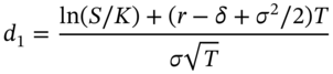
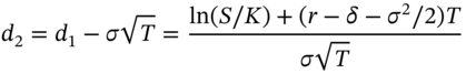
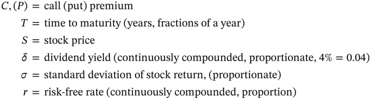
APPENDIX 28: BLACK–SCHOLES AND THE GREEKS
The Black–Scholes formula for the price of a European call option on a stock which pays a continuous dividend yield at a rate ![]() (per annum) can be obtained by taking the Black–Scholes equation for an option on a non-dividend paying stock and replacing
(per annum) can be obtained by taking the Black–Scholes equation for an option on a non-dividend paying stock and replacing ![]() by
by ![]() .
.
Call and Put Premia: European Options, Dividend Paying Stock
For calls and puts on a stock (index) paying continuous dividends:
Since ![]() then:
then:
Delta:
![]()
Call Delta: ![]()
Put Delta: ![]()
Gamma:
![]()

Vega:
![]()
Rho:
![]() (for both a dividend paying and non-dividend paying stock)
(for both a dividend paying and non-dividend paying stock)
Call: ![]()
Put: ![]()
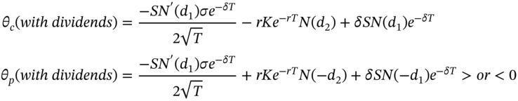
Theta
![]() :
:
a. Non-dividend paying stock
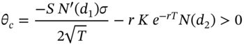
Note that T = ‘time to maturity’ and therefore as the call gets closer to maturity, T falls. It can be shown that as the option approaches the maturity date, theta increases and the call premium becomes more sensitive to changes in ‘time’ – the call loses time-value more quickly.
b. Dividend paying stock
In the above formulas time is measured in years. For example, if ![]() , then the change in price of the option over 2 trading days is
, then the change in price of the option over 2 trading days is ![]() (16 cents).
(16 cents).
Theta is usually negative for a long position in an option – as time passes the option becomes less valuable – this is ‘time decay’. However, there are some (pathological) cases where theta can be positive – for example, for an ITM European put on a non-dividend paying stock or an ITM European call on a currency that pays a high interest rate.
If we set ![]() in any of the above formulas then we will obtain the Black–Scholes ‘Greeks’ for an option on a non-dividend paying stock.
in any of the above formulas then we will obtain the Black–Scholes ‘Greeks’ for an option on a non-dividend paying stock.
Options on Foreign Currency and Options on Futures
The above formulas for options on dividend paying stocks can be easily adapted to apply to European options on foreign currencies and European options on futures. The changes required are:
Foreign currency options:
- Replace
 with the foreign interest rate
  ,
,  = spot exchange rate and
  = volatility of the spot FX-rate. There are two rhos, one with respect to the domestic interest rate which is given above and one with respect to the foreign interest rate
  which is given by:
![]()
Call: ![]()
Put: ![]()
Futures option:
- Replace
 by
by  (so that
  ‘disappears’ from the definition of
  and
and  ), replace
  by
by  (the futures price, with the same expiration date as the option) and
  is the volatility of the futures price.
EXERCISES
Question 1
Briefly explain the concept of the delta of a portfolio of options (on the same underlying asset).
Question 2
What is the vega of an option and why is it useful?
Question 3
How does the gamma of a long call vary as the price of the underlying (stock) changes around the strike price? What are the risk management implications after selling an ATM call with a high gamma?
Question 4
Suppose portfolio-A, which consists of several options, is delta neutral but has a gamma of minus 300. A call option-Z on the same underlying stock is available which has a delta of 0.62 and a gamma of 1.5.
How can you use option-Z and any stocks you might buy or sell to make your overall portfolio gamma and delta neutral?
Question 5
You are a trader (market maker) who supplies clients with whatever calls or puts they want to buy or sell. At the end of the trading day you have a portfolio of (long and short) calls and put options on Microsoft stock and on AT&T stock. Carefully explain to your risk manager what additional trades you are immediately going to do, to hedge your current options positions over the next 3 days. What are the costs in setting up your hedged postion?
Question 6
You hold a Portfolio-A of options with the following Greeks:
(![]() is the vega of the option). Option ‘Z’ is available with
is the vega of the option). Option ‘Z’ is available with ![]() ,
, ![]() ,
, ![]() and option ‘Y’ is available with
and option ‘Y’ is available with ![]() ,
, ![]() and
and ![]() .
.
Explain how you can combine options A, Y and Z to give a portfolio which is ‘gamma, vega and delta neutral’.
Question 7
In the BOPM how do you calculate the gamma of an option at t = 0?
NOTES
- 1 The gamma of an option is a similar concept to the convexity of a bond.
- 2 From an earlier chapter, the percentage hedging error is the bank debt (loan outstanding) at T less the invested call premium, expressed as a percentage of the initial call premium, that is

- 3 An estimate of theta at
 = 0 can also be obtained (for
  ) using other elements in the tree, for example:
  or
or  . There are many different ways of estimating the Greeks using, for example, forward, backward and central differences (see Chapter 47).