CHAPTER 30
Other Options
Aims
- To show how a corporate's debt and equity can be valued using options theory.
- To examine different types of equity warrants, which are long-term options on a company's stock.
- To examine quantos which are long-term equity options written on foreign stocks but with the payout in the home currency.
- To show how an equity collar enables a portfolio manager to set an upper and lower limit on the performance of her existing equity portfolio. If this is achieved at zero ‘up-front’ cost then it is known as a zero cost collar or a risk reversal.
In this chapter we show how the debt and equity of a firm can be valued using options theory. Then we examine equity warrants, which are stock options ‘attached to’ bonds. Finally, we discuss how an equity collar places a floor price and a ceiling price on a stock (or stock portfolio).
30.1 CORPORATE EQUITY AND DEBT
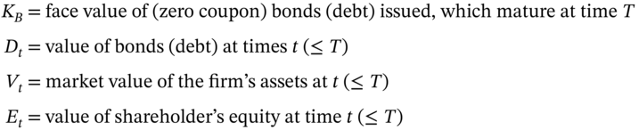
Merton (1974) and Black–Scholes (1973) noted that the debt and equity of a firm can be valued using options theory. Suppose a corporation has two sources of finance, debt ![]() and equity
and equity ![]() . If the value of the firm's assets
. If the value of the firm's assets ![]() at time t, exceeds the face value of debt (bonds) outstanding
at time t, exceeds the face value of debt (bonds) outstanding ![]() then the equity holders have a positive stake in the firm. On the other hand, if
then the equity holders have a positive stake in the firm. On the other hand, if ![]() the bondholders may put the firm into liquidation. In this case the equity holders receive nothing but they can ‘walk away’, as they have limited liability and any other assets they own cannot be taken by the liquidator. The payoff to equity holders is therefore like a call option with a payoff, max
the bondholders may put the firm into liquidation. In this case the equity holders receive nothing but they can ‘walk away’, as they have limited liability and any other assets they own cannot be taken by the liquidator. The payoff to equity holders is therefore like a call option with a payoff, max ![]() . We have:
. We have:
Case A: Solvency at Time T
If the value of the firm ![]() exceeds the face value
exceeds the face value ![]() of the bonds
of the bonds ![]() , the bonds are worth
, the bonds are worth ![]() and the equity is worth
and the equity is worth ![]() .
.
Case B: Insolvency at Time T
If ![]() then the bonds are worth
then the bonds are worth ![]() and
and ![]() .
.
For the above two states, the payoffs to equity and debt holders are (see Figure 30.1):
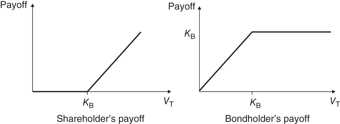
FIGURE 30.1 Payoffs
The value of the equity is therefore like a European call on the value of the firm's assets with a strike price of ![]() . If we assume that
. If we assume that ![]() follows a geometric Brownian motion (GBM), then value of the firm's equity
follows a geometric Brownian motion (GBM), then value of the firm's equity ![]() (at
(at ![]() ) is given by the Black–Scholes formula for a European call option:
) is given by the Black–Scholes formula for a European call option:
Now consider the market value of the debt at time T. The equity holders can ‘hand over’ the firm to the bondholders if ![]() . The bondholders have written a put option on the assets of the firm. The payoff to the bondholders consists of a short put plus an amount
. The bondholders have written a put option on the assets of the firm. The payoff to the bondholders consists of a short put plus an amount ![]() (at time T). The value of the debt today
(at time T). The value of the debt today ![]() equals the PV of the face value of the bonds,
equals the PV of the face value of the bonds, ![]() less the value of the put held by the equity shareholders:
less the value of the put held by the equity shareholders:
where ![]() is the current value of a European put on the firm's assets with a strike price of
is the current value of a European put on the firm's assets with a strike price of ![]() . The call and put premia
. The call and put premia ![]() and
and ![]() are given by the Black–Scholes formulas. Note that the current value of the debt
are given by the Black–Scholes formulas. Note that the current value of the debt ![]() is less than the value of a risk-free bond
is less than the value of a risk-free bond ![]() because of the risk of default represented by the written put
because of the risk of default represented by the written put ![]() because if default occurs, the bondholders will not be paid the full face value of their bonds.
because if default occurs, the bondholders will not be paid the full face value of their bonds.
30.1.1 Pricing
It was Merton (1973) who provided a closed-form solution for pricing the corporate bond ![]() . Since the value of the firm is assumed to follow a Brownian motion, the equation for
. Since the value of the firm is assumed to follow a Brownian motion, the equation for ![]() has similar features to the Black–Scholes formula. The market price of the risky corporate debt is:
has similar features to the Black–Scholes formula. The market price of the risky corporate debt is:
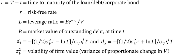
The Merton model also provides an equation for the yield spread (over risk-free T-bonds) that should be charged to a corporate borrower:
The predictions of the model are quite intuitive. In particular, the spread should increase the higher is either the leverage ratio or the volatility of the firm's assets. An extended version of the above approach can be used in measuring credit default risk in the following way.1 If Dt and Vt could be accurately measured then (30.4) can be inverted to solve for the implied volatility ![]() of the firm's total assets. Suppose
of the firm's total assets. Suppose ![]() . Then assuming normality, there is only a 5% chance that the value of the firm V will fall below
. Then assuming normality, there is only a 5% chance that the value of the firm V will fall below ![]() . Suppose the current value of the firm is $100m and its outstanding debt is $80m. Then our option's model implies that there is a 5% chance of the firm going into ‘financial distress’, over the life of the debt (i.e. the period
. Suppose the current value of the firm is $100m and its outstanding debt is $80m. Then our option's model implies that there is a 5% chance of the firm going into ‘financial distress’, over the life of the debt (i.e. the period ![]() ). Unfortunately
). Unfortunately ![]() and
and ![]() are not easily measured for a levered firm (e.g. which has non-marketable bank loans) so further analysis is needed to make the model operational.
are not easily measured for a levered firm (e.g. which has non-marketable bank loans) so further analysis is needed to make the model operational.
It is worth noting that we have taken a fairly simple example, where all debt matures on the same date (i.e. a zero-coupon bond). Valuing coupon paying corporate bonds is obviously more difficult since each coupon payment represents a put option and if an ‘early’ put option is exercised, the ‘later’ put options are worthless. Also, corporate bonds often contain convertible or call provisions (i.e. the payoffs are path dependent). This means that it may not be technically possible to derive closed-form solutions and other methods such as binomial trees, Monte Carlo simulation and numerical solution of PDEs are required – these techniques are discussed in other parts of the book.
30.2 WARRANTS
Equity warrants are one of the oldest manifestations of options. They are call options written by a firm on its own stock. Initially they arose because a firm issuing long-term bonds felt the bonds would be more attractive to investors (and therefore could be issued at a lower yield) if warrants were ‘attached’ to the bond. The warrants give the bondholder the opportunity to purchase the firm's stock at some time in the future, at a price fixed today.2 If the firm does well in the future and its stock price increases, then the warrants would be ‘in-the-money’ and could be exercised at a profit by the warrant holder.
Equity warrants are sometimes referred to as ‘equity kickers’ since they give the holder the opportunity to participate in the ‘upside’ if the firm is successful in the future but also allow the investor the relative security of a corporate bondholder (who receive payments ahead of stockholders). These warrants are often ‘stripped’ from the bonds and traded separately on stock exchanges. Warrants are also sometimes given out by companies, either in payment for underwriters' fees or as part of a company's executive remuneration package – they are then referred to as executive stock options. The maturity of a warrant could be anything from about 2 to 12 years (or more) and hence warrants are ‘long-term’ options carrying the credit risk of the issuing firm.
30.2.1 Valuing European Warrants
European warrants can only be exercised on a certain day. They can be valued much like ordinary European stock options. However, if a warrant is exercised, then the company has to issue more stocks and hence increase the number of stocks outstanding. This ‘dilution’ does not occur when an exchange traded option is exercised, as the option writer has to purchase stocks on the NYSE.
Suppose a company has ![]() stocks outstanding with current price
stocks outstanding with current price ![]() so the value of the company to equity holders is
so the value of the company to equity holders is ![]() . Today the company issues
. Today the company issues ![]() (European) warrants and each warrant allows the holder to purchase one stock from the company at time T, at a strike price of K. The value of the company does not change on announcement of the warrant issue (assuming any future cash flow from the warrants does not change the underlying profitability of the company by improving incentives or lowering costs of production). After the announcement of the warrant issue, the value of the company remains at
(European) warrants and each warrant allows the holder to purchase one stock from the company at time T, at a strike price of K. The value of the company does not change on announcement of the warrant issue (assuming any future cash flow from the warrants does not change the underlying profitability of the company by improving incentives or lowering costs of production). After the announcement of the warrant issue, the value of the company remains at ![]() as the future exercise of the options (and consequent ‘dilution’) is already reflected in the current stock market price,
as the future exercise of the options (and consequent ‘dilution’) is already reflected in the current stock market price, ![]() – the market is said to be ‘efficient’. If the stock price at maturity of the warrant is
– the market is said to be ‘efficient’. If the stock price at maturity of the warrant is ![]() , the value of the equity in the company will be
, the value of the equity in the company will be ![]() (with or without the warrants).
(with or without the warrants).
If the warrants are exercised at ![]() , there is a cash inflow to the company of
, there is a cash inflow to the company of ![]() and the market value of the company's equity increases from
and the market value of the company's equity increases from ![]() to
to ![]() , while the number of stocks outstanding rises to
, while the number of stocks outstanding rises to ![]() . The stock price immediately after exercise is therefore:
. The stock price immediately after exercise is therefore:
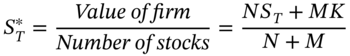
If exercised, the payoff to the warrant holder is ![]() . Substituting for
. Substituting for ![]() from (30.6) and rearranging:
from (30.6) and rearranging:
The warrant payoff is equivalent to holding ![]() regular call options. The current price of the stock is
regular call options. The current price of the stock is ![]() which using Black–Scholes gives a call premium
which using Black–Scholes gives a call premium ![]() , so the value of each warrant is:
, so the value of each warrant is:
So the total cost of the warrant issue is ![]() . The total value of the company's equity will decline by
. The total value of the company's equity will decline by ![]() as soon as the decision to issue the warrants is announced and therefore the stock price will fall by
as soon as the decision to issue the warrants is announced and therefore the stock price will fall by ![]() at
at ![]() .
.
A bond with a warrant attached will sell at a lower yield (higher price) than a conventional bond. This makes the ‘bond-plus-warrant’ an attractive source of finance for small firms with growth potential. The bond-plus-warrant will have lower coupon payments than a conventional bond (with the same maturity and tenor) and therefore involves less cash outflow for the firm but also gives the warrant holder a share in high profits should these occur in the future.
‘Warrant’ is often used as a generic term for an option with a long maturity date. As well as warrants on individual stocks there are also warrants (often on stock indices) written by third parties (e.g. Morgan Stanley, Citigroup) which are sold to investors and then traded on an exchange (e.g. American Stock Exchange), rather than OTC.
30.2.2 Quanto
A quanto is a long maturity option based on a foreign stock index such as the Nikkei 225 and traded (say) on the American Stock Exchange (AMEX). For example, if ![]() a long call (quanto) on the Nikkei 225 gives a US holder a payoff at expiration of
a long call (quanto) on the Nikkei 225 gives a US holder a payoff at expiration of ![]() . However, the special feature of a quanto is that at the time the option is purchased, the contract fixes the rate of exchange between the yen and the US dollar which will apply at maturity of the quanto. Hence there is no exchange risk.
. However, the special feature of a quanto is that at the time the option is purchased, the contract fixes the rate of exchange between the yen and the US dollar which will apply at maturity of the quanto. Hence there is no exchange risk.
For example, if the payoff ![]() on the Nikkei 225 is equivalent to ¥20,000 and the exchange rate agreed at
on the Nikkei 225 is equivalent to ¥20,000 and the exchange rate agreed at![]() is 100 Yen/USD, then the USD payoff is $200. Thus a quanto allows a US investor to speculate on future value of the Nikkei 225 index without incurring any exchange rate risk.
is 100 Yen/USD, then the USD payoff is $200. Thus a quanto allows a US investor to speculate on future value of the Nikkei 225 index without incurring any exchange rate risk.
30.3 EQUITY COLLAR
Suppose you hold stocks (with price ![]() ) but are worried about a fall in prices and want to secure a minimum value for your portfolio, then today you could buy a put, with a low strike price
) but are worried about a fall in prices and want to secure a minimum value for your portfolio, then today you could buy a put, with a low strike price ![]() . The ‘stock+put’ allows unlimited upside potential, should stock prices rise. However, if you are willing to forego some of the upside potential, you could sell a call with a high strike price,
. The ‘stock+put’ allows unlimited upside potential, should stock prices rise. However, if you are willing to forego some of the upside potential, you could sell a call with a high strike price, ![]() . The cash received from selling the call can be used to offset the cost of the put. The payoff to this strategy is an equity collar – it establishes a minimum and maximum value for your existing stocks (Figure 30.2).
. The cash received from selling the call can be used to offset the cost of the put. The payoff to this strategy is an equity collar – it establishes a minimum and maximum value for your existing stocks (Figure 30.2).
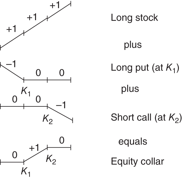
FIGURE 30.2 Equity collar
An equity collar has the same payoff profile as a bull spread which we discussed in Chapter 17. The key difference is that the bull spread is constructed using only options but an equity collar starts with a stock and then uses options to provide a floor and a ceiling on the future value of the stocks.
The payoff from the equity collar is given in detail in Table 30.1 for three possible outcomes for the stock price at maturity T, of the options. The lower bound for the payoff on the collar is ![]() and the upper bound is
and the upper bound is ![]() . The net cost of establishing the collar is:
. The net cost of establishing the collar is:
TABLE 30.1 Equity collar payoffs
|
|
|
|
|
| Long stocks |
|
|
|
| Long put (K1) |
|
0 | 0 |
| Short call (K2) | 0 | 0 |
|
| Payoff |
|
|
|
| Profit |
|
|
|
If the stock price at maturity lies between the two strike prices, then the profit and the breakeven stock price are:
30.3.1 Zero-cost Collar (Risk Reversal, Range Forward)
If the strike prices are chosen so that the put and call premia exactly offset each other (i.e. ![]() ) then the collar can be set up at zero cost – this is called a risk reversal, range forward or simply, a zero-cost collar. By definition a ‘risk reversal’ has
) then the collar can be set up at zero cost – this is called a risk reversal, range forward or simply, a zero-cost collar. By definition a ‘risk reversal’ has ![]() and hence
and hence ![]() (Equation (30.11)). Suppose we chose a floor level
(Equation (30.11)). Suppose we chose a floor level ![]() and hence via Black–Scholes
and hence via Black–Scholes ![]() is fixed, then a zero-cost collar requires:
is fixed, then a zero-cost collar requires:
We ‘invert’ the Black–Scholes formula for ![]() and solve (30.12) for
and solve (30.12) for ![]() (e.g. by using Excel's ‘Solver’). Once you have chosen
(e.g. by using Excel's ‘Solver’). Once you have chosen ![]() , you must accept whatever value that arises from Equation (30.12) for
, you must accept whatever value that arises from Equation (30.12) for ![]() , which ensures
, which ensures ![]() .
.
The beauty of the zero-cost collar is that an investor holding stocks can fix a maximum and minimum value for her stocks at no ‘up-front’ cost. There is a guaranteed minimum value for the stocks and yet the investor can still share in some of the upside should stock prices rise. However, this is not a ‘something for nothing’ outcome – financial markets never give you that! True, the (zero cost) collar gives you a floor value – which you like. But the ‘hidden cost’ is the fact that it eliminates the possibility of very large upside gains (which you might get if you only held the stocks plus the put, but this would involve a cost equal to the put premium).
In a zero-cost collar ![]() implies that you can only choose one of the strikes, either for the call or the put. Also the zero-cost collar will probably involve at least one strike price for which there may not be exchange traded options available. For example, suppose the portfolio manager chooses
implies that you can only choose one of the strikes, either for the call or the put. Also the zero-cost collar will probably involve at least one strike price for which there may not be exchange traded options available. For example, suppose the portfolio manager chooses ![]() , for the put which using Black–Scholes gives
, for the put which using Black–Scholes gives ![]() . For a zero-cost collar the portfolio manager now requires
. For a zero-cost collar the portfolio manager now requires ![]() . But suppose inverting the Black–Scholes equation for the call premium (e.g. using Excel's ‘Solver’) gives
. But suppose inverting the Black–Scholes equation for the call premium (e.g. using Excel's ‘Solver’) gives ![]() . Since there is no traded call option with
. Since there is no traded call option with ![]() then either the collar will not quite be ‘zero cost’ or OTC options must be used.
then either the collar will not quite be ‘zero cost’ or OTC options must be used.
30.4 SUMMARY
- Options theory can be used to value a corporate's equity and debt (i.e. bank loans and bonds issued). The payoff to equity holders is like a call option. The value of the equity in the firm is therefore equal to the value of a European call on the firm's assets, with a strike price equal to the face value of the bonds (debt).
- Bondholders have written a put option on the firm's assets. Hence the value of the firm's debt is equal to the market value of the bonds issued, less the value of the put held by the equity holders (with a strike price equal to the face value of the bonds).
- Warrants are ‘long maturity’ options on a stock with maturities ranging from 2 to 12 years. Warrants are often initially attached to bonds, which have a lower yield than plain vanilla bonds. For investors, the warrant combines the relative safety of a conventional bond but allows upside potential if the stock price rises. The warrant is like a call option on the value of the firm and can be priced using a variant of the Black–Scholes formula.
- A quanto is an option with a payoff at maturity which depends on the level of a foreign stock index but with payments made in the home currency, based on an exchange rate which is fixed when the quanto is purchased. Quantos therefore provide a low cost method for portfolio managers to take a position in foreign stocks (or stock indices) without incurring FX risk.
- An equity collar establishes a minimum and maximum value for stocks (or stock portfolio) already held by an investor. An equity collar consists of the initial stock holdings, together with a long put with a low strike price
 and a short call with a high strike price
  . If the collar has zero ‘up-front’ cost (that is,
  ) it is called a zero-cost collar (risk reversal).
EXERCISES
Question 1
An investment manager holds a portfolio worth $4,351,700, which can be thought of as 10,000 shares of a single stock worth ![]() (which pays no dividends). Her performance will be evaluated in 78 days
(which pays no dividends). Her performance will be evaluated in 78 days ![]() and she would like to establish a maximum and minimum profit over the remaining period until the evaluation is made.
and she would like to establish a maximum and minimum profit over the remaining period until the evaluation is made.
She finds that a zero-cost equity collar can be constructed by buying a put with ![]() and selling a call with
and selling a call with ![]() , both with maturity
, both with maturity ![]() . The continuously compounded risk-free rate is 4.14% p.a. and the volatility of the stock is 15% p.a.
. The continuously compounded risk-free rate is 4.14% p.a. and the volatility of the stock is 15% p.a.
Use Black–Scholes (with Excel) to show that ![]() so the zero-cost collar is fairly priced. Show your calculated values for
so the zero-cost collar is fairly priced. Show your calculated values for ![]() etc.
etc.
Question 2
A fund already holds stocks and a zero-cost equity collar is constructed by buying a put with ![]() for a price
for a price ![]() and selling a call with
and selling a call with ![]() and price
and price ![]() .
.
Calculate and explain the payoffs if the stock price at maturity ends up at either ![]() or 435 or 415.
or 435 or 415.
Question 3
The current price of stock-Z is ![]() (which pays no dividends). Ms Sparkle, a fund manager, originally invested $800,000 in stock-Z and is now worth $1m. Over the next year Ms Sparkle is worried about increased volatility in the stock market and wants to lock in a minimum value for her holdings in stock-Z of $900,000, in 1 year's time. Options traders' current view is that the volatility of stock-Z is
(which pays no dividends). Ms Sparkle, a fund manager, originally invested $800,000 in stock-Z and is now worth $1m. Over the next year Ms Sparkle is worried about increased volatility in the stock market and wants to lock in a minimum value for her holdings in stock-Z of $900,000, in 1 year's time. Options traders' current view is that the volatility of stock-Z is ![]() p.a. and the risk-free rate is 3% (continuously compounded).
p.a. and the risk-free rate is 3% (continuously compounded).
What will it cost Ms Sparkle to insure her portfolio? What is the cost in relation to the current value of Ms Sparkle's holdings of stock-Z?
Question 4
Given the scenario in question 3, Ms Sparkle thinks the cost of providing a floor is rather expensive, as it takes a big chunk out of her past gains of $200,000. She decides to sell a call today with strike ![]() .
.
- What is now the net cost of Ms Sparkle's position? Qualitatively, will Ms Sparkle's stocks and options positions give her a profit after 1 year, if stock-Z is worth $115 in a year's time?
- If Ms Sparkle decides today that she wants a zero-cost collar, what strike price will her written call have and what will her profit/loss be if in 1 year's time the stock-Z is worth $130. Ex-post, will Ms Sparkle be happy that she went for a zero-cost collar?
Question 5
Explain why the value of the equity in a firm is like a European call on the value of the firm's assets with a strike price equal to the face value of the bonds ![]() issued by the firm. Consider the outcomes for equity and debt holders if the firm is solvent or insolvent at maturity of the bonds.
issued by the firm. Consider the outcomes for equity and debt holders if the firm is solvent or insolvent at maturity of the bonds.
Question 6
Explain why an equity warrant is like a call option.
Question 7
How does a ‘quanto’ differ from a plain vanilla call option?