CHAPTER 13
T-bond Futures
Aims
- To examine contract details for UK Gilt futures and US T-bond futures including the conversion factor, the cheapest-to-deliver bond and wild card play.
- To determine the optimal number of T-bond futures contracts for hedging.
- To determine the fair price of a T-bond futures contract using cash-and-carry arbitrage.
- To analyse speculative strategies using T-bond futures. This includes spread trades and altering the effective duration of a bond portfolio to take advantage of market timing strategies.
Some of the practical details of T-bond futures are quite intricate. A long T-bond futures position allows the holder to take delivery of a long maturity T-bond at expiration of the futures contract. As with all futures contracts, T-bond futures can be used for speculation, arbitrage, and hedging. Hedging allows the investor to eliminate price risk of her bond portfolio.
For example, suppose Ms Bond holds $20m in (cash market) 20-year T-bonds and she fears a rise in long-term yields over the next 6 months. Ms Bond should hedge by shorting (selling) T-bond futures. If long rates do subsequently rise, the price of her cash-market T-bonds will fall but so does the futures price. Hence, she can close out her short futures position at a profit by buying back the T-bond futures at a lower price. The profit from the futures position compensates for the loss in value of her cash market position in T-bonds.
If Ms Bond wants to act as a speculator and she forecasts that long-term yields will fall in the future then today she would purchase T-bond futures contracts. If yields fall, then the futures price will rise and she can close out her long position in T-bond futures at a higher price – hence making a speculative profit.
Ms Bond gains leverage by purchasing the futures contract rather than purchasing T-bonds in the cash market (with her own funds) – because she only has to provide a relatively small initial futures margin (and not the full price of the cash market bond). Transactions costs (e.g. bid–ask spreads, clearing, and brokerage fees) in the futures market might also be lower than those in the cash market.
Naked speculative positions in T-bond futures are highly risky, therefore speculators often use spread trades. For example, they might purchase one T-bond futures contract with a long maturity date and simultaneously sell another T-bond futures with a short maturity date. This provides possible speculative profits but also reduces risk compared with an outright long or short position in T-bonds.
13.1 CONTRACT SPECIFICATIONS
T-bond futures contracts written on a number of government bonds are traded on several exchanges. The most liquid contracts are on US T-bond futures (CBOT) quoted in US dollars. There are also Euro-Bond futures – for example, on French and German bonds (‘Bunds’) which are both quoted in euros, and also UK Gilt futures (quoted in sterling) – all traded on NYSE-Euronext. Somewhat less liquid T-bond futures are those on Japanese government bonds, traded on NYSE-Euronext and in Tokyo.
13.1.1 UK Long Gilt Futures Contract
Details of the UK Long Gilt Future (on NYSE-EURONEXT) are given in Table 13.1. The bond deliverable in the contract is a ‘notional bond’ with a 4% coupon (with a maturity between 8.75 and 13 years). Surprisingly, this notional 4% bond does not actually exist! However, as we shall see, it provides a benchmark from which to calculate the price of possible bonds for delivery (which do exist).
TABLE 13.1 UK Long Gilt Futures (Euronext-LIFFE)
| Contract size | £100,000 nominal, notional Gilt with 4% coupon |
| Delivery months | March / June / September / December |
| Quotation | Per £100 nominal |
| Tick size (value) | £0.01 (£10) |
| Last trading day | 11 a.m., 2 business days prior to the last business day in the month |
| Delivery day | Any business day in the delivery month (seller's choice) |
| Settlement | List of deliverable Gilts published by the exchange with maturities between 8.75–13 years |
| Margin requirements | Initial margin £2,000, spread margin £250 (determined by the exchange) |
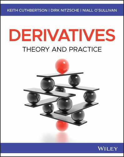
The seller of the futures contract can decide the exact delivery date (within the delivery month) and exactly which bond she will deliver (from a limited set, designated by the exchange). In fact, the seller will select a bond which is known as the ‘cheapest-to-deliver’ (CTD). The CTD bond can be shown to depend on the ‘conversion factor’ (CF) for each possible deliverable bond. (These concepts are explained below.)
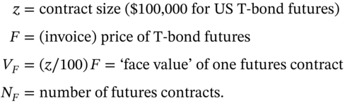
The futures contract size is for delivery of ![]() (face value) T-bonds and futures price quotes are expressed per £100 nominal (of deliverable T-bonds). The tick size is £0.01 per £100 nominal (e.g. 1-tick is a move from £95 to £95.01) – hence the tick value is £10 per contract
(face value) T-bonds and futures price quotes are expressed per £100 nominal (of deliverable T-bonds). The tick size is £0.01 per £100 nominal (e.g. 1-tick is a move from £95 to £95.01) – hence the tick value is £10 per contract ![]() .
.
13.1.2 US ‘Classic’ and ‘Ultra’ T-bond Futures Contracts
The principles underlying these futures contracts (traded on the CBOT) are very similar to those for the UK gilt-futures contract, except price quotes are in 1/32nd of 1% (see Table 13.2). Expiration months are March, June, September, and December. The last trading day is the business day prior to the last 7 days of the expiry month. The first delivery day is the 1st business day of the delivery month but delivery can take place on any business day in the delivery month.
TABLE 13.2 US ‘classic’ T-bond futures (CBOT)
| Contract size | £100,000 nominal, notional US Treasury Bond with 6% coupon |
| Delivery months | March / June / September / December |
| Quotation | Per $100 nominal |
| Tick size (value) | 1/32 ($31.25) |
| Last trading day | 7 working days prior to last business day in expiry months |
| Delivery day | Any business day in the delivery month (seller's choice) |
| Settlement | Any US Treasury bond maturing at least 15 years from the contract month (or not callable for 15 years) and with less than 25 years to maturity. |
| Margins | $5,000 initial, $4,000 maintenance (decided by the exchange) |
| Trading hours | 8 a.m. to 2 p.m. – Central Time |
| Daily price limits | 96 points ($3,000) |
Note that the notional bond deliverable in the futures contract is assumed to be a 6%-coupon bond. However, in practice the person with a ‘short’ futures position can choose from around 30 different eligible bonds to deliver (which have coupons different from 6% and the CF adjusts the delivery price to reflect the type of bonds actually delivered).
For the ‘classic’ futures contract the T-bonds delivered must have at least 15 years to maturity2 and less than 25 years to maturity (from the first day of the delivery month).3 There are also futures on 2, 5 and 10-year T-notes, which only differ from the T-bond futures contract in the maturity of the T-notes which can be delivered in the contract. As with most futures contracts, delivery rarely takes place but it is the possibility of delivery and hence arbitrage profits which keeps the T-bond futures price in line with the spot/cash market price of T-bonds.
13.2 CONVERSION FACTOR AND CHEAPEST-TO-DELIVER
Before discussing hedging strategies we need to be clear about the use of the conversion factor (CF) and the concept of the cheapest-to-deliver (CTD) bond. We do so with respect to the US T-bond futures contract but similar principles apply to UK Gilt futures. There are a wide variety of bonds with over 15 years to maturity which can be delivered by the investor who is short T-bond futures. These will have different maturities and coupon payments and hence different values for CF and the CTD.
13.2.1 Conversion Factor (CF)
This section assumes the reader is largely familiar with the pricing of bonds in the spot market and the conventions used in calculating accrued interest (see Cuthbertson and Nitzsche 2008). The CF adjusts the price of the actual bond to be delivered, by assuming it has a 6% yield, which makes it equivalent to the notional 6% bond in the futures contract.
When computing the CF the maturity of the underlying bond is defined as the maturity on the first day of the delivery month. For example, if we assume the actual delivery date is 11 September 2018 and the underlying bond matures on 15 February 2038, then the maturity period used in the calculation of CF is 1 September (i.e. not 11 September) to 15 February 2038.
The CF is best understood using a specific example. To simplify matters we assume the counterparty who is short the futures contract does not yet hold a bond for delivery, so we are going to calculate the CF and CTD bond at the maturity date of the futures contract (=T).
Consider an actual 20-year US T-bond, paying semi-annual coupons of 8% (i.e. $4 per 6 months), with ![]() (6-month) periods to maturity (see Example 13.3). If the yield to maturity on this 8%-coupon bond is assumed to be 6% p.a. then its ‘fair’ or ‘theoretical’ price would be $123.1 (per $100 nominal) which gives a conversion factor
(6-month) periods to maturity (see Example 13.3). If the yield to maturity on this 8%-coupon bond is assumed to be 6% p.a. then its ‘fair’ or ‘theoretical’ price would be $123.1 (per $100 nominal) which gives a conversion factor ![]() . In essence the deliverable bond (with an 8% coupon) is worth 1.231 times as much as the notional 6% coupon bond (trading at par and hence with
. In essence the deliverable bond (with an 8% coupon) is worth 1.231 times as much as the notional 6% coupon bond (trading at par and hence with ![]() ).
).
The conversion factor adjusts the price of the actual bond to be delivered, relative to the notional 6% coupon bond in the futures contract:
The conversion factor will differ for bonds with different coupon payments and different maturities. The CF for any specific deliverable bond will change over time simply because the maturity date of the deliverable bond gets closer (although it will always exceed 15 years, otherwise it will cease to be an eligible bond). In calculating the CF the CBOT assumes the yield curve is flat at 6%. But in practice this is rarely (if ever) the case. This means that the ‘true price’ of the deliverable bond, which should be priced using spot rates (see Cuthbertson and Nitzsche 2008) will not equal that used in the calculation of the CF. Hence, there will usually be eligible bonds for delivery that are actually cheaper than the ‘cheapest-to-deliver’ bond.
Let us now consider the cash amount received by a trader (Ms Short) who is short T-bond futures, when she delivers the underlying bond at maturity ![]() . Let
. Let ![]() be the futures settlement price (on the ‘position day’ – see below). When Ms Short delivers the 8%-coupon, 20 year bond she will receive:
be the futures settlement price (on the ‘position day’ – see below). When Ms Short delivers the 8%-coupon, 20 year bond she will receive:
Ms Short's receipts at settlement

Note that ![]() is the ‘settlement price’ at
is the ‘settlement price’ at ![]() (and not the price initially agreed at the outset of the futures contract).
(and not the price initially agreed at the outset of the futures contract). ![]() is the accrued interest at
is the accrued interest at ![]() and is a fraction of the next coupon payment on the bond delivered against the futures contract. For example, if the maturity date
and is a fraction of the next coupon payment on the bond delivered against the futures contract. For example, if the maturity date ![]() of the futures is 11 September 2017 and the deliverable bond matures on 15 February 2038, then the deliverable bond has semi-annual coupons each year on 15 February and 15 August. Assume there are 184 days between 15 August and 15 February. The short therefore delivers a bond at T = 11 September 2017, which already has 27 days of accrued interest. Hence the long must pay the short for this loss of accrued interest of
of the futures is 11 September 2017 and the deliverable bond matures on 15 February 2038, then the deliverable bond has semi-annual coupons each year on 15 February and 15 August. Assume there are 184 days between 15 August and 15 February. The short therefore delivers a bond at T = 11 September 2017, which already has 27 days of accrued interest. Hence the long must pay the short for this loss of accrued interest of ![]() .
.
13.2.2 Cheapest-to-Deliver
Suppose it is now ![]() (= 11 September 2017) and there are three bonds designated by CBOT for actual delivery in September whose CF are 1.044, 1.033, and 1.065. In practice, the calculation of the CTD bond is quite complex but a rough idea of the CTD bond can be obtained by choosing that bond with the smallest raw basis:
(= 11 September 2017) and there are three bonds designated by CBOT for actual delivery in September whose CF are 1.044, 1.033, and 1.065. In practice, the calculation of the CTD bond is quite complex but a rough idea of the CTD bond can be obtained by choosing that bond with the smallest raw basis:
where ![]() is the spot (‘clean’) price an eligible bond for delivery,
is the spot (‘clean’) price an eligible bond for delivery, ![]() is the settlement futures price and
is the settlement futures price and ![]() is the conversion factor of a deliverable bond.
is the conversion factor of a deliverable bond.
Table 13.3 shows the calculation of the raw basis for three deliverable bonds. The final column indicates that Bond-C is the CTD. Although it is often the case that the bond actually delivered by the short is the CTD, nevertheless this is not always so since the seller may wish to preserve the duration of her own bond portfolio or provide a bond, other than the CTD, in order to minimise her tax bill. We now examine how Equation (13.1) for the raw basis arises. At settlement the short receives:
TABLE 13.3 The CTD bond
| Deliverable bonds (maturity) | Spot price ($) | Conversion factor |
Raw basis |
|
112-4 (112.125) | 1.044 | 0.156 |
|
112-8 (112.25) | 1.033 | 1.461 |
|
114-8 (114.25) | 1.065 | 0.029 |
Notes: F(September-futures) = 107-8 (107.25)
where ![]() is the accrued interest. The conversion factor adjusts the T-bond futures price for the fact that the deliverable bond has a coupon different from the notional 6% bond (stated in the T-bond futures contract). The 8%-coupon bond actually delivered would have a higher price when its coupons are discounted at the notional 6%. To purchase the actual deliverable bond in the cash market, the short will pay:
is the accrued interest. The conversion factor adjusts the T-bond futures price for the fact that the deliverable bond has a coupon different from the notional 6% bond (stated in the T-bond futures contract). The 8%-coupon bond actually delivered would have a higher price when its coupons are discounted at the notional 6%. To purchase the actual deliverable bond in the cash market, the short will pay:
Hence, the net cost to the short of providing the deliverable 8%-coupon bond is just the raw basis defined above:
13.3 HEDGING USING T-BONDS
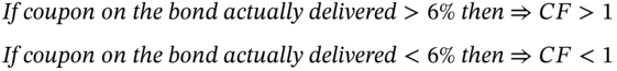
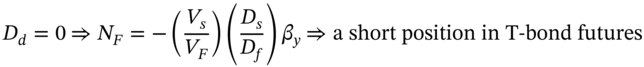
Today, if Ms Bond is (net) long in US T-bonds ![]() with a positive portfolio duration
with a positive portfolio duration ![]() and fears a fall in bond prices, then to hedge she will short T-bond futures. Conversely, if she wishes to purchase bonds in the future and is worried that cash market T-bond prices will rise (i.e. yields will fall) then today she should buy T-bond futures. The optimal number of futures contracts
and fears a fall in bond prices, then to hedge she will short T-bond futures. Conversely, if she wishes to purchase bonds in the future and is worried that cash market T-bond prices will rise (i.e. yields will fall) then today she should buy T-bond futures. The optimal number of futures contracts ![]() is given by the duration-based hedge ratio (see Appendix 13.A):
is given by the duration-based hedge ratio (see Appendix 13.A):
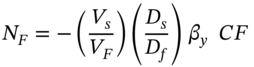
Equation (13.5) assumes ![]() is defined using continuously compounded rates for
is defined using continuously compounded rates for ![]() and
and ![]() . But if
. But if ![]() and
and ![]() are quoted yields to maturity (e.g. using discrete semi-annual compounding) then we use modified duration
are quoted yields to maturity (e.g. using discrete semi-annual compounding) then we use modified duration ![]() , in place of
, in place of ![]() in the above equations for
in the above equations for ![]() .
.
13.3.1 Portfolio Duration
For illustrative purposes assume a fund manager has two T-bonds in her portfolio, with market values ![]() in Bond-1 and
in Bond-1 and ![]() in Bond-2, so that
in Bond-2, so that ![]() . The portfolio duration
. The portfolio duration ![]() of her cash-market position is:
of her cash-market position is:
where ![]() ,
, ![]() and
and ![]() is the duration of bond-i, for
is the duration of bond-i, for ![]() . Using portfolio duration to calculate
. Using portfolio duration to calculate ![]() assumes a parallel shift in the yield curve and small changes in yields (e.g. 25 bps) – otherwise the hedging error could be large.
assumes a parallel shift in the yield curve and small changes in yields (e.g. 25 bps) – otherwise the hedging error could be large.
13.3.2 Hedging a T-bond Portfolio
Consider a US pension fund manager (Ms Bond) on 1 May who wishes to hedge her portfolio of Corporate bonds (or T-bonds) with market value ![]() 4 and portfolio duration
4 and portfolio duration ![]() . Ms Bond fears a rise in interest rates over the next 3 months (i.e. 1 May to 1 August) and if this occurs the value of her cash-market bond portfolio will fall. The
. Ms Bond fears a rise in interest rates over the next 3 months (i.e. 1 May to 1 August) and if this occurs the value of her cash-market bond portfolio will fall. The ![]() of the CTD bond is 1.12 (Table 13.4A). For a portfolio of corporate bonds this would be a cross-hedge, as the corporate bonds are hedged using T-bond futures.
of the CTD bond is 1.12 (Table 13.4A). For a portfolio of corporate bonds this would be a cross-hedge, as the corporate bonds are hedged using T-bond futures.
TABLE 13.4A Hedging a US bond portfolio
| Cash market – 1 May | Futures (September delivery) – 1 May |
| Market value of bond portfolio, |
CF of CTD bond = 1.12 Size of one contract, z = $100,000 Futures Price, F0 = 103-16 ($103.5) V F = z(F0/100) = $103,500 |
| Duration, |
Duration (futures), Df = 18 Tick value 1/32 equals $31.25 |
Ms Bond, on 1 May, sells September T-bond futures contracts and assuming a parallel shift in the yield curve ![]() and no complications of accrued interest:
and no complications of accrued interest:

Suppose interest rates rise between 1 May and 1 August (Table 13.4B). Her cash-market bond portfolio falls by 5% to $1,045,000 – a capital loss of $55,000. But the futures price falls by 4 points from ![]() to
to ![]() and the gain on the short futures position is
and the gain on the short futures position is ![]() . The hedge shows a small loss of $3,000 on an initial cash-market value of about $1m (i.e. about 0.3%). The unhedged portfolio would have lost $55,000 (i.e. about 5.5%).
. The hedge shows a small loss of $3,000 on an initial cash-market value of about $1m (i.e. about 0.3%). The unhedged portfolio would have lost $55,000 (i.e. about 5.5%).
TABLE 13.4B Hedge outcome
| Cash market – 1 August | Futures (September delivery) – 1 August |
| Loss on bond portfolio = $1,100,000 – $1,045,000 = $55,000 |
September futures: Gain on 13 short futures = NFz(F0 – F1)/100 = 13($100,000)(4)/100 = $52,000 = 13 × 128 ticks × $31.25 = $52,000 |
13.4 HEDGING: FURTHER ISSUES
13.4.1 Cross Hedge: Corporate Bond Portfolio
Suppose company-XYZ is going to raise funds by issuing corporate bonds in 6 months' time, after the legal details of the bond issue are completed. The treasurer of company-XYZ may be worried by the possibility of a rise in long-term interest rates over the next 6 months, which will raise the cost of issuing corporate bonds. Company-XYZ therefore hedges by shorting T-bond futures.
When hedging corporate bonds, it is important to estimate the relationship between ![]() (the change in the corporate bond yield) and
(the change in the corporate bond yield) and ![]() (the yield on the deliverable bond in the T-bond future contract), since these may change by different amounts over the hedge period.
(the yield on the deliverable bond in the T-bond future contract), since these may change by different amounts over the hedge period.
Regression techniques can be used but results may be subject to error, as changes in corporate ‘specific risk’ (e.g. IT failures, results of patent applications, environmental issues, default) will affect changes in the corporate bond yield ![]() – whereas changes in
– whereas changes in ![]() (government T-bond yields) should be largely unaffected by these ‘corporate risks’.
(government T-bond yields) should be largely unaffected by these ‘corporate risks’.
13.4.2 PVBP, Convexity, and Perturbation Analysis
Instead of using the duration-based hedge ratio we could obtain the same result using the ‘price value of a basis point’ (PVBP). This requires the calculation of the PVBP for the cash-market bond portfolio to be hedged and the PVBP for the US T-bond futures contract. This method usually uses the duration approximation for the change in T-bond prices and therefore assumes a parallel shift in the yield curve and small changes in interest rates.
Alternatively, we can calculate the PVBP of the cash-market (spot) bond portfolio using the ‘duration + convexity’ approximation (for a parallel shift in the spot yield curve of 1 bp):
where ![]() is the cash-market convexity,
is the cash-market convexity, ![]() proportion of the total bond portfolio held in bond-i and
proportion of the total bond portfolio held in bond-i and ![]() .
.
Alternatively, we can use the ‘full’ (present value) pricing formula when considering the effect of a large change in interest rates on the ‘total’ change in the cash-market value of a T-bond portfolio – this will implicitly incorporate the convexity of the bonds. The ‘full valuation’ method can be done for either parallel or non-parallel shifts in spot yields – as spot rates might change by different amounts.
13.4.2.1 Non-parallel Shifts
We can also calculate the change in dollar value of one futures contract, ![]() using
using ![]() where the change is calculated with respect to changes in the spot yields which determine (a) the price of the deliverable bond
where the change is calculated with respect to changes in the spot yields which determine (a) the price of the deliverable bond ![]() and (b) the (future) value of any coupon payments
and (b) the (future) value of any coupon payments ![]() . The number of futures in the hedge is then:
. The number of futures in the hedge is then:

This is a form of perturbation analysis because we choose the size of the change in each spot interest rate along the yield curve and then calculate the impact on the numerator and denominator in Equation (13.9).
13.4.3 Hedging the Market Risk of an Underpriced Corporate Bond
In Chapter 6 we discussed how a hedge fund that buys underpriced stocks can hedge the market risk of the stocks by shorting stock index futures. Consider a similar situation where Ms Bond today, buys what she believes are underpriced corporate bonds (of several companies). She might believe the corporate bonds are underpriced because the rating agencies (and the average bond trader) have given the bond an A-rating but her assessment of their default risk would suggest a higher AA-rating.
She therefore expects a rise in the market price of the bond (even if risk-free government bond yields stay constant), as ‘market participants’ come to realise that the corporate bond is actually less risky than they first thought. Then she can close out her long corporate bond position at a profit.
However, Ms Bond is exposed to changes in long-term (risk-free) T-bond yields. If long-term risk-free yields increase, this will cause a fall in the cash market price of her corporate bonds, which may more than offset the gains she makes when the ‘credit risk underpricing’ is corrected. To hedge against future changes in T-bond yields, Ms Bond should short![]() , T-bond futures, today:
, T-bond futures, today:
where ![]() is the total dollar amount held in her portfolio of underpriced cash-market corporate bonds which have a portfolio duration of
is the total dollar amount held in her portfolio of underpriced cash-market corporate bonds which have a portfolio duration of ![]() . If the risk-free T-bond rate increases, then the T-bond futures price will fall and the profit after closing out the futures will just compensate for any loss in value of the cash-market bond position – solely due to changes in risk-free T-bond yields.
. If the risk-free T-bond rate increases, then the T-bond futures price will fall and the profit after closing out the futures will just compensate for any loss in value of the cash-market bond position – solely due to changes in risk-free T-bond yields.
Ms Bond can then capture any future rise in corporate bond prices due to the correction of the ‘credit risk’ mispricing. However, her portfolio of underpriced corporate bonds is still subject to any (residual) ‘specific risk’ (e.g. bankruptcy, regulatory changes, IT failures, reputational damage, etc.) of the bond issuers. The hedge using T-bond futures does not protect the ‘mispriced’ corporate bond portfolio from specific risks – but overall, specific risk may be small in a well-diversified corporate bond portfolio.
13.4.3.1 Long-Short Bond Portfolio
As in the case of underpriced and overpriced stocks, a bond trader might take a long position in ‘underpriced’ corporate bonds and short-sell ‘overpriced’ corporate bonds.5 The dollar amount of cash-market bonds held long ![]() or short (
or short (![]() ), determine the portfolio durations
), determine the portfolio durations ![]() and hence the number of T-bond futures to go long and short, using Equation (13.10). The net position in futures contracts depends on the sign of
and hence the number of T-bond futures to go long and short, using Equation (13.10). The net position in futures contracts depends on the sign of ![]() , but this ensures the long-short bond speculator is then hedged against parallel shifts in the yield curve, while she waits for the mispricing of the cash-market bonds to be corrected.
, but this ensures the long-short bond speculator is then hedged against parallel shifts in the yield curve, while she waits for the mispricing of the cash-market bonds to be corrected.
13.4.4 Risks in the Hedge
A hedged bond portfolio will not provide a perfect hedge because:
- the hedge period (e.g. 3 months from May to August) may not match the maturity date of the futures contract (e.g. September contract) – this gives rise to basis risk.
- calculating price changes in futures markets are subject to error, in part because it is difficult to ascertain the CTD bond (and hence its duration).
- shifts in the yield curve may not be parallel (there may be twists in the yield curve), so we cannot always assume duration or duration plus convexity provides a good approximation to changes in T-bond cash-market prices.
- If we are hedging a corporate bond portfolio then the change in the value of the corporate bonds due to changes in risk-free T-bond yields can be hedged using T-bond futures but changes in corporate bond prices due to any change in (residual) specific/credit risk will not be hedged.
However, academic studies find that hedging using T-bond futures can reduce price risk, with the duration based hedge ratio performing particularly well. Hedging cash-market positions in corporate bonds using T-bond futures is also found to be effective, even though this is a cross-hedge and involves possible changes in credit risk.
13.5 MARKET TIMING
Suppose a trader Ms Bond currently holds a bond portfolio and over the next month she expects interest rates to fall sharply. Today, to take advantage of this interest rate forecast she might move out of low duration bonds and into high duration bonds, because the latter will rise in price more than the former. However, this is likely to be costly because it involves ‘high’ transaction costs of selling low duration bonds and buying high duration bonds – and then reversing these trades in one month's time (when she returns to her ‘normal long-run’ position in bonds).
A less costly strategy is to continue to hold the original cash market bond portfolio and alter the effective duration of the portfolio using T-bond futures. Suppose, ![]() = portfolio duration of Ms Bond's cash-market T-bonds,
= portfolio duration of Ms Bond's cash-market T-bonds, ![]() = duration of the T-bond deliverable in the futures contract and
= duration of the T-bond deliverable in the futures contract and ![]() = Ms Bond's target (desired) duration. The number of futures contracts required to achieve a desired duration
= Ms Bond's target (desired) duration. The number of futures contracts required to achieve a desired duration ![]() is (see Appendix 13.A):
is (see Appendix 13.A):
where we usually assume that ![]() and hence
and hence ![]() .6 The formula for
.6 The formula for ![]() can be used in a market timing strategy. Suppose you are long a cash-market bond portfolio (so
can be used in a market timing strategy. Suppose you are long a cash-market bond portfolio (so ![]() and
and ![]() are positive) then:
are positive) then:
- If you expect a rise in yields (i.e. fall in bond prices) and therefore require a lower desired duration
 , then today, sell
 T-bond futures.
 - If you expect a fall in yields (i.e. rise in bond prices) and therefore require a higher desired duration
 , then today, buy
 T-bond futures.
13.6 WILD CARD PLAY
There is another practical issue to discuss as regards the US T-bond futures contracts and that is the strategy known as Wild Card Play. On the CBOT, trading in T-bond futures ceases at 3 p.m. (EST) while actual T-bonds are traded until 5 p.m. (EST) and the ‘short’ in the futures contract has until early evening to issue the clearing house with notice of intention to deliver. If the notice is issued, the invoice price of the T-bond futures is calculated on the basis of the settlement price (i.e. average of quoted prices just before the close of trading). However, the short can wait and see if she can purchase an eligible bond for delivery, at a lower price in the cash market. To see how this is possible we have to closely examine the delivery process for T-bond futures. Delivery is a 3-day process and involves:
- Position Day:
The short notifies the clearing house of intention to deliver, two business days later.
- Notice of Intention Day:
The clearing house assigns a trader who is long, to accept delivery. The short is now obligated to deliver the next business day.
- Delivery Day:
Bonds are delivered (with the last possible delivery day being the business day prior to the last 7 days in the delivery month).
This delivery process can give rise to a Wild Card Play by the short on any ‘position day’. If the cash-market price of bonds falls between 3 p.m. and 5 p.m., the short buys the ‘low price’ CTD bond in the cash market and issues a notice of intention to deliver, knowing that on delivery she will receive the ‘high’ futures settlement price determined as of 3 p.m. that day. However, if the bond price does not decline, she can wait until the next day and repeat this strategy (until the final business day before the final delivery day in the month). In essence, the short has an implicit option that can be exercised during the delivery month, while the long has increased risk because she does not know the exact bond that will be delivered.
There is also a quality or switching option for the short, since she can deliver a variety of eligible bonds. Even if she holds a specific bond against delivery on her short futures position, nevertheless if the yield curve shifts she may choose to deliver another yet cheaper bond. The timing option applies when the bond held for delivery by the short pays a coupon (rate) that exceeds the cost of financing her cash-market bond position (i.e. the repo rate). Then it is better if the short delays delivery. There is also an end of the month option held by the short, since the last trading day for the T-bond futures contract is the eighth-to-last business day. The futures settlement price is fixed in over this period, but the short still has the option to announce her intention to deliver on any day up to the penultimate business day. She can therefore wait to see if cash-market bond prices fall over this period and deliver a ‘low’ price bond if one becomes available.
All of these embedded options available to the person holding a short T-bond futures position should lead to a lower futures price – in order to compensate the long, for the increased risk. But it is thought that most of the time these options do not distort the cash-and-carry arbitrage relationship. However, these embedded options for the short do make it more difficult to accurately calculate both the optimal hedge ratio and the futures price based on the cash-and-carry approach.
13.7 PRICING T-BOND FUTURES
13.7.1 Futures Price on Deliverable Zero-coupon Bond
Suppose today is time ![]() and the futures contract matures at
and the futures contract matures at ![]() , so the time to maturity is
, so the time to maturity is ![]() . The underlying asset to be delivered at maturity
. The underlying asset to be delivered at maturity ![]() is a single zero-coupon bond. Today, we can borrow at
is a single zero-coupon bond. Today, we can borrow at ![]() and purchase the underlying bond for a price
and purchase the underlying bond for a price ![]() in the cash market and later deliver it against the short futures position. The usual risk free arbitrage argument ensures that:
in the cash market and later deliver it against the short futures position. The usual risk free arbitrage argument ensures that:
The implied repo rate (![]() ) is the return from selling the futures at
) is the return from selling the futures at ![]() for
for ![]() and simultaneously buying the underlying bond at
and simultaneously buying the underlying bond at ![]() , so that
, so that ![]() (compound rate). In this case, risk-free arbitrage is possible if
(compound rate). In this case, risk-free arbitrage is possible if ![]() does not equal
does not equal ![]() , the cost of financing the arbitrage strategy using the actual repo market.
, the cost of financing the arbitrage strategy using the actual repo market.
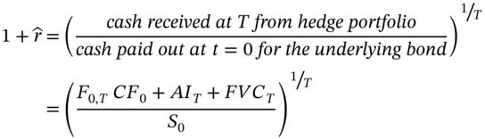
13.7.2 Futures Price on Deliverable Coupon Paying Bond
In practice there is not a futures contract on a zero-coupon bond. As we saw in Chapter 3 if we ignore some important practical issues, the fair price (at ![]() ) of a T-bond futures contract using cash-and-carry arbitrage is:
) of a T-bond futures contract using cash-and-carry arbitrage is:
where ![]() is the invoice price of the cash-market bond (i.e. the ‘clean price’ plus accrued interest),
is the invoice price of the cash-market bond (i.e. the ‘clean price’ plus accrued interest), ![]() is the present value of any coupon payments (on the deliverable bond) between today and the maturity date
is the present value of any coupon payments (on the deliverable bond) between today and the maturity date ![]() of the futures contract and
of the futures contract and ![]() is the (continuously compounded) spot yield (for maturity
is the (continuously compounded) spot yield (for maturity ![]() ). Note that the T-bond futures price can also be written
). Note that the T-bond futures price can also be written ![]() , where the future value at
, where the future value at ![]() of the coupon payments is
of the coupon payments is  .
.
Unfortunately, in practice it is difficult to accurately calculate the fair T-bond futures price. This is because of the flexibility of the short's decision over the delivery date ![]() and the precise choice of the CTD bond and hence its invoice price
and the precise choice of the CTD bond and hence its invoice price ![]() .
.
First, note that the cost of creating a synthetic futures contract is the cost of buying the underlying cash-market bond at ![]() using borrowed funds, which accrues to a debt of
using borrowed funds, which accrues to a debt of ![]() at maturity
at maturity ![]() (of the futures contract). The cost-of-carry is offset by the
(of the futures contract). The cost-of-carry is offset by the ![]() coupons
coupons ![]() received from the cash-market bond at times
received from the cash-market bond at times ![]() from today. When these coupons are reinvested at the (expected) risk-free rates
from today. When these coupons are reinvested at the (expected) risk-free rates ![]() (between
(between ![]() and
and ![]() ) they have a future value at
) they have a future value at ![]() of:
of:
The no-arbitrage futures price is then:
where ![]() is the interest rate over the period (
is the interest rate over the period (![]() ). Considering the additional complexities of the conversion factor, accrued interest etc., the futures price for a contract which matures at
). Considering the additional complexities of the conversion factor, accrued interest etc., the futures price for a contract which matures at ![]() (and has time
(and has time ![]() to maturity) is:
to maturity) is:
Let's examine this from a more practical point of view, which requires some additional points to be made. Suppose it is 1 July 2017. The yield curve is flat and ![]() (3% p.a., continuously compounded). You are deciding whether cash-and-carry arbitrage is possible with the September T-bond futures contract, which has a known maturity date T = 11 September (Figure 13.1).
(3% p.a., continuously compounded). You are deciding whether cash-and-carry arbitrage is possible with the September T-bond futures contract, which has a known maturity date T = 11 September (Figure 13.1).
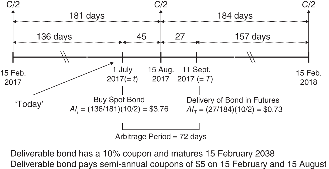
FIGURE 13.1 Pricing a T-bond futures contract
By buying a cash-market T-bond on 1 July and carrying it forward to 11 September, you create a synthetic T- bond future, since the T-bond can be delivered against the futures contract. Assume the CTD bond is a 10%-coupon T-bond which pays semi-annual coupons of $5 each year, on 15 August and 15 February and matures on 15 February 2038. It has a CF of 1.22.
Today at ![]() = 1 July to the maturity of the futures, the deliverable bond pays one coupon of
= 1 July to the maturity of the futures, the deliverable bond pays one coupon of ![]() on 15 August, which when invested over 27 days is expected to accrue to a future value at time T of:
on 15 August, which when invested over 27 days is expected to accrue to a future value at time T of:
On 1 July, borrowing at the risk-free (repo rate) ![]() and purchasing the bond in the cash market for an invoice price
and purchasing the bond in the cash market for an invoice price![]() , leads to an amount owing at
, leads to an amount owing at ![]() = 11 September, of
= 11 September, of ![]() (i.e. purchase cost plus the repo interest cost). Therefore at
(i.e. purchase cost plus the repo interest cost). Therefore at ![]() , the net cost-of-carry in the cash market is:
, the net cost-of-carry in the cash market is:
But the above strategy creates a synthetic T-bond future since it ensures that the bond purchased in the cash market on 1 July is available for delivery against the futures contract at ![]() = 11 September. At maturity of the futures
= 11 September. At maturity of the futures ![]() , the invoice price the long pays the short for delivery of the underlying T-bond is the quoted price of
, the invoice price the long pays the short for delivery of the underlying T-bond is the quoted price of ![]() plus accrued interest7:
plus accrued interest7:
![]() is the accrued interest (between 15 August and T = 11 September) on the CTD bond delivered at
is the accrued interest (between 15 August and T = 11 September) on the CTD bond delivered at ![]() (see Figure 13.1).
(see Figure 13.1). ![]() is a proportion of the next coupon which accrues on 15 February 2018.
is a proportion of the next coupon which accrues on 15 February 2018.
Since the actual futures contract and the synthetic futures both deliver one bond at ![]() then the cost today must be equal, otherwise risk-free arbitrage profits would be possible. Hence equating (13.15) and (13.16):
then the cost today must be equal, otherwise risk-free arbitrage profits would be possible. Hence equating (13.15) and (13.16):
The no-arbitrage (fair) futures price is:
where ![]() is the cash-market bond price (i.e. clean price
is the cash-market bond price (i.e. clean price ![]() plus accrued interest
plus accrued interest ![]() payable when initially purchased at time t). If there are no coupon payments over the arbitrage period (i.e.
payable when initially purchased at time t). If there are no coupon payments over the arbitrage period (i.e. ![]() ), no accrued interest (
), no accrued interest (![]() ) and the deliverable bond is the one specified in the futures contract (
) and the deliverable bond is the one specified in the futures contract (![]() ), then not surprisingly the above formula for
), then not surprisingly the above formula for ![]() reduces to that for the futures price on a zero-coupon bond, namely
reduces to that for the futures price on a zero-coupon bond, namely ![]() .
.
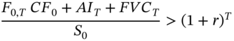
13.7.3 Arbitrage
Profitable risk-free arbitrage would ensue if the invoice price of the futures ![]() received at
received at ![]() , exceeds the cost of the synthetic futures (
, exceeds the cost of the synthetic futures (![]() ) at
) at ![]() .8 Today at t, the arbitrageur borrows an amount
.8 Today at t, the arbitrageur borrows an amount ![]() at a cost of
at a cost of ![]() (the repo rate), purchases the bond and simultaneously sells T-bond futures. The amount owed at
(the repo rate), purchases the bond and simultaneously sells T-bond futures. The amount owed at ![]() , the expiry of the futures contract is:
, the expiry of the futures contract is:
Hence the net (cash-market) cost at ![]() is
is ![]() , but the arbitrageur receives a larger amount
, but the arbitrageur receives a larger amount ![]() . This arbitrage creates additional demand for cash-market bonds so
. This arbitrage creates additional demand for cash-market bonds so ![]() increases and sales of bond futures will reduce
increases and sales of bond futures will reduce ![]() until the equality in (13.17) is restored and the equilibrium futures price is given by Equation (13.18).
until the equality in (13.17) is restored and the equilibrium futures price is given by Equation (13.18).
However, the arbitrage strategy is not completely risk-free because the coupon payments received from the cash market T-bond have to be re-invested at interest rates which are unknown at ![]() (1 July). At
(1 July). At ![]() , the best guess of the reinvestment rate for any coupon receipts would be the implied forward rate – and to lock in this rate would require a strip of FRAs. Hence cash-and-carry arbitrage only provides an approximate formula for the T-bond futures price.
, the best guess of the reinvestment rate for any coupon receipts would be the implied forward rate – and to lock in this rate would require a strip of FRAs. Hence cash-and-carry arbitrage only provides an approximate formula for the T-bond futures price.
13.8 T-BOND FUTURES SPREADS
A spread is a long position in one asset and a short position in another (similar) asset. A T-bond futures spread can be used to speculate on twists or parallel shifts in the yield curve. For example, a trader Ms Bond could undertake a spread trade by buying a T-bond futures (which delivers a bond with at least 15 years to maturity) and simultaneously selling a 10-year T-bond in the cash market (i.e. which has a different maturity/duration to the CTD bond in the futures). She might then profit after a change in interest rates as the futures price and cash-market prices change by different amounts (because their underlying durations are different). For example, if all interest rates fall by 1% she would gain more on the long futures than she loses on the short bond position, because the duration of the futures is higher than the duration of the cash-market bond.
A spread trade is less risky than holding just a naked futures position – although potential profits are also less. However, such a strategy would have to take account of margin requirements and any ‘haircuts’ on short-sales of bonds in the cash market. A spread trade may be less costly if two futures contracts are used, with different maturities.
13.8.1 Turtle Trade: Arbitrage Profits
13.8.1.1 Buying the Spread
First, let us examine how an arbitrage ‘June-September’ T-bond futures spread position can be used to exploit any mispricing along the yield curve (Figure 13.2). Suppose at ![]() (1 April 2017) we:
(1 April 2017) we:
- buy a T-bond futures which matures at
 (1 June 2017)
 - sell a T-bond futures which matures at
 (1 September 2017) and
 - you borrow money at the forward repo rate
 (applicable between June and September) by selling the June-Eurodollar futures on 1 April.
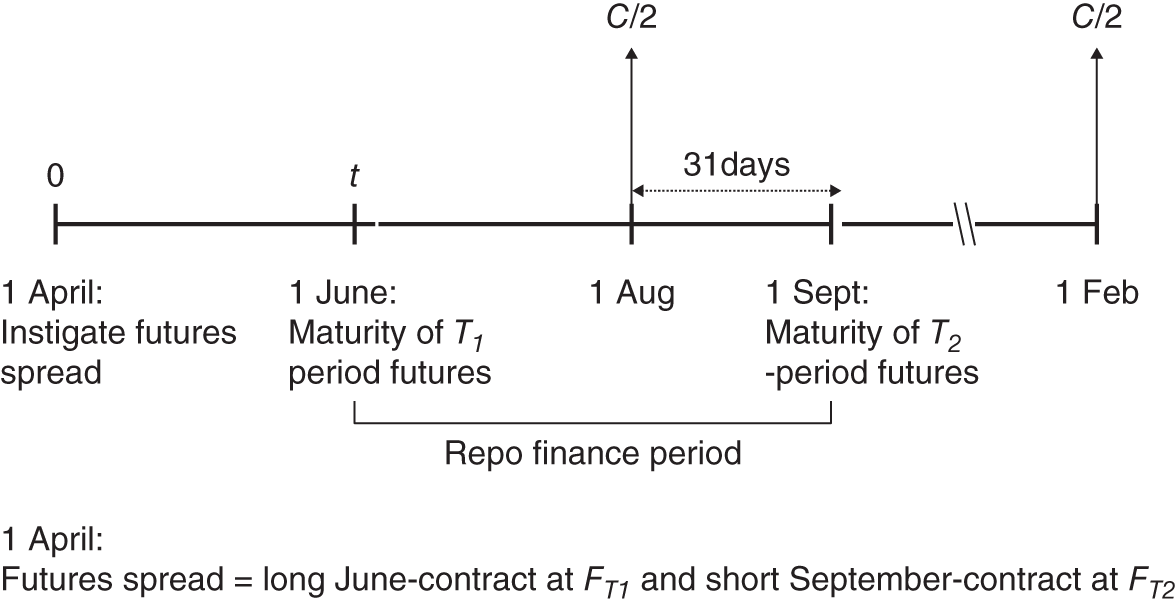
FIGURE 13.2 T-bond futures spreads
We are buying the spread (i.e. we buy the nearby T-bond futures contract). When the nearby T-bond futures contract matures we take delivery of the eligible bond (which matures on 1 August 2038, say) and pay ![]() (plus any accrued interest,
(plus any accrued interest, ![]() ) with finance raised by borrowing at the (forward) repo rate.
) with finance raised by borrowing at the (forward) repo rate.
We then ‘carry’ this cash market bond until 1 September when it is delivered against the short September-futures position and we receive ![]() (plus any accrued interest
(plus any accrued interest ![]() , arising from the underlying bond's next coupon payment on 1 February 2018). The (compound) return from this long-spread strategy9 is the implied repo rate
, arising from the underlying bond's next coupon payment on 1 February 2018). The (compound) return from this long-spread strategy9 is the implied repo rate ![]() :
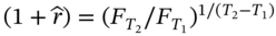
:
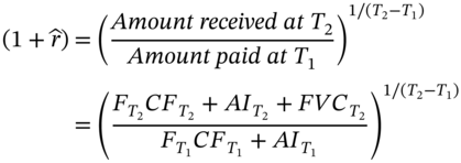
where ![]() is the (future) value of any coupons paid on the ‘carried’ cash-market bond on 1 August 2017, compounded to T = 1 September 2017. Note that the implied repo rate is a forward rate. If the implied repo rate
is the (future) value of any coupons paid on the ‘carried’ cash-market bond on 1 August 2017, compounded to T = 1 September 2017. Note that the implied repo rate is a forward rate. If the implied repo rate ![]() (say) exceeds the cost of borrowing at the actual forward repo rate
(say) exceeds the cost of borrowing at the actual forward repo rate ![]() (applicable between 1 June and 1 September), then a long arbitrage spread trade undertaken on 1 April is guaranteed to be profitable.
(applicable between 1 June and 1 September), then a long arbitrage spread trade undertaken on 1 April is guaranteed to be profitable.
The actual repo borrowing rate is the forward rate ![]() , when viewed from
, when viewed from ![]() (1 April 2017). How can we ‘lock-in’ this forward rate on 1 April? Today we sell June-Eurodollar futures contracts at
(1 April 2017). How can we ‘lock-in’ this forward rate on 1 April? Today we sell June-Eurodollar futures contracts at ![]() . When we close out the Eurodollar futures in June, the effective cost (between June and September) is the implied forward rate
. When we close out the Eurodollar futures in June, the effective cost (between June and September) is the implied forward rate ![]() ).10 You use the cash inflow on 1 June from closing out several short Eurodollar futures contracts, to pay
).10 You use the cash inflow on 1 June from closing out several short Eurodollar futures contracts, to pay ![]() (plus accrued interest) for delivery of the eligible T-bond in the maturing June T-bond futures. Hence if the implied (forward) repo rate from buying the spread is
(plus accrued interest) for delivery of the eligible T-bond in the maturing June T-bond futures. Hence if the implied (forward) repo rate from buying the spread is ![]() and the cost of borrowing is
and the cost of borrowing is ![]() (= 4.16%, the actual forward repo rate), we undertake the following turtle trade on 1 April:
(= 4.16%, the actual forward repo rate), we undertake the following turtle trade on 1 April:
Turtle trade
Buy the T-bond futures spread and sell June-Eurodollar futures.
When the implied repo rate (i.e. the ‘percentage return’ on the T-bond spread trade) exceeds the actual (forward) repo cost of borrowing, an overall profit will be made on the turtle trade.
13.8.1.2 Selling the Spread
Suppose we have the reverse position on 1 April, namely the implied repo rate ![]() , the actual (forward) repo rate. Then you sell the T-Bond spread, so on 1 April:
, the actual (forward) repo rate. Then you sell the T-Bond spread, so on 1 April:
- sell the June T-bond futures
- buy the September T-bond futures and
- you lend money at the forward repo rate
 (applicable between June and September) by buying the June Eurodollar futures on 1 April.
Selling the June T-bond futures and buying the September T-bond futures is equivalent to borrowing at the forward rate ![]() . By buying the Eurodollar futures is equivalent to lending at
. By buying the Eurodollar futures is equivalent to lending at ![]() . Hence the trade results in an arbitrage profit of 0.3%.
. Hence the trade results in an arbitrage profit of 0.3%.
The above strategy is an intermarket spread since it involves two T-bond futures contracts which mature at different dates but are on the same underlying asset (i.e. a cash-market T-bond). They are not risk-free trades because of the difficulty of ascertaining the CTD bond in each contract and uncertainty surrounding the reinvestment rate of any coupons paid.
13.9 SUMMARY
- Contract details for T-bond futures are necessarily complex because of the use of the conversion factor (CF), the cheapest-to-deliver bond (CTD), and Wild Card Play.
- Holders of cash-market T-bonds can hedge their position, using the duration based hedge ratio to determine the number of T-bond futures contracts
 to short. Conversely, to hedge a future purchase of cash-market T-bonds, you buy
 T-bond futures, today.
 - T-bond futures contracts are useful for hedging a corporate bond portfolio, even though corporate bond prices and T-bond futures prices might not be perfectly positively correlated (e.g. due to changes in credit risk of the corporate bond) – hence there will be some hedging error. This is a cross hedge.
- Even when hedging a T-bond portfolio with T-bond futures a perfect hedge is not possible because of basis risk (i.e. the cash-market T-bond prices and futures prices do not move perfectly together). This is exacerbated by non-parallel shifts in the yield curve.
- T-bond futures are used to increase (decrease) the effective duration of an existing cash-market bond portfolio, when the investor forecasts yields to fall (rise). This is a market timing strategy.
- Speculation with T-bond futures often involves spread trading where the speculator takes a long position in nearby T-bond futures and a short position in T-bond futures with a longer maturity date (or vice versa). Spread trades can be used to speculate on parallel shifts and twists in the yield curve.
- The fair price of a T-bond futures contract can be determined using cash-and-carry arbitrage.
- Profitable arbitrage opportunities with T-bond futures are usually expressed in terms of the implied repo rate. If the implied repo rate differs from the actual repo rate (i.e. the cost of lending/borrowing funds), then profitable arbitrage is possible.
APPENDIX 13.A: HEDGING: DURATION AND MARKET TIMING
First (for illustrative purposes), consider a cash-market (spot) position in two bonds, where ![]() = (invoice) price of bond-i and
= (invoice) price of bond-i and ![]() = number of bonds-i held (
= number of bonds-i held (![]() if held long or
if held long or ![]() if short-sold). The dollar value and change in the cash-market T-bond portfolio is:
if short-sold). The dollar value and change in the cash-market T-bond portfolio is:
Cash Market
where we use the duration approximation, ![]() . For a parallel shift in spot yields
. For a parallel shift in spot yields ![]() , then:
, then:
where ![]() ,
, ![]() for
for ![]() and
and ![]() is the portfolio duration of the cash-market bond portfolio.
is the portfolio duration of the cash-market bond portfolio.
T-bond futures
The change in value of a portfolio consisting of ‘cash-market T-bonds+T-bond futures’ (ignoring accrued interest) is:
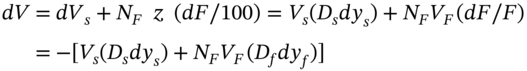
Assume the relationship between the change in the YTM of the cash-market T-bonds and the change in the yield (on the deliverable bond) in the T-bond futures contract is ![]() , then:
, then:
To fully hedge your cash-market T-bond portfolio we set ![]() , hence:
, hence:
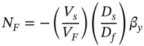
which is sometimes referred to as the minimum variance hedge ratio.
Effective Duration and Market Timing
Suppose a trader holds a cash-market (spot) T-bond portfolio and she wants to change the effective duration of the portfolio to some desired level ![]() , using T-bond futures contracts. The desired change
, using T-bond futures contracts. The desired change![]() in her cash-market T-bond portfolio is:
in her cash-market T-bond portfolio is:
Equating (13.A.5) and (13.A.7):11
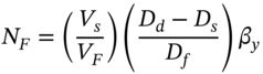
The cash-market T-bond position could be either net long or short – depending on the sign of ![]() – and the cash-market portfolio duration could be positive or negative depending on the value of
– and the cash-market portfolio duration could be positive or negative depending on the value of ![]() . For the moment assume
. For the moment assume ![]() and
and ![]() are both positive. Then (13.A.8) gives the required number of futures contracts to achieve a ‘desired duration’:
are both positive. Then (13.A.8) gives the required number of futures contracts to achieve a ‘desired duration’:
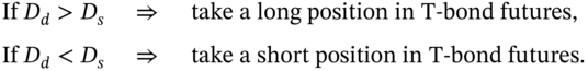
Hence, to increase (decrease) the effective duration of an underlying (long) cash-market bond portfolio (with ![]() ), we go long (short) T-bond futures. This makes sense because if interest rates subsequently fall, then you make profits both from the cash market bond portfolio and the long T-bond futures contracts – this is equivalent to increasing the duration of the cash-market bond portfolio and is a form of ‘market timing’. If your forecasts are correct then you will make more profit by taking the long futures position rather than just holding your cash-market bond portfolio.
), we go long (short) T-bond futures. This makes sense because if interest rates subsequently fall, then you make profits both from the cash market bond portfolio and the long T-bond futures contracts – this is equivalent to increasing the duration of the cash-market bond portfolio and is a form of ‘market timing’. If your forecasts are correct then you will make more profit by taking the long futures position rather than just holding your cash-market bond portfolio.
Note that (13.A.6) the minimum variance hedge ratio is a special case of (13.A.8), where the desired duration, ![]() :
:
APPENDIX 13.B: IMPLIED REPO RATE AND ARBITRAGE
The implied repo rate is another way of determining whether risk-free arbitrage profits are possible. The implied repo rate is the return from buying the underlying cash-market T-bond at ![]() for the invoice price
for the invoice price ![]() and simultaneously selling the futures for delivery at
and simultaneously selling the futures for delivery at ![]() . The return or implied repo rate
. The return or implied repo rate![]() (using discrete compounding) is:
(using discrete compounding) is:
where ![]() = futures price set at
= futures price set at ![]() for payment at
for payment at ![]() (when the underlying bond is delivered) and the conversion factor is
(when the underlying bond is delivered) and the conversion factor is ![]() . The arbitrageur holds the underlying bond and receives coupon payments which can be reinvested over the period
. The arbitrageur holds the underlying bond and receives coupon payments which can be reinvested over the period ![]() to
to ![]() to give a future value
to give a future value ![]() . The accrued interest on the deliverable bond at maturity of the futures contract is
. The accrued interest on the deliverable bond at maturity of the futures contract is ![]() . The cash-market bond has an invoice price of
. The cash-market bond has an invoice price of ![]() and this is financed by borrowing at the (actual) repo rate
and this is financed by borrowing at the (actual) repo rate ![]() , at
, at ![]() .
.
It is easy to see using (13.B.1) that if ![]() then:
then:
Part of the reason for using the implied repo rate to determine possible arbitrage profits is that it is straightforward to compare the implied repo rate with the quoted repo rate (cost of borrowing funds). Using (13.B.2), the elimination of any arbitrage profits implies the fair (no-arbitrage) T-bond futures price is:
If we replace the discrete compound rate ![]() by the continuously compounded rate
by the continuously compounded rate ![]() then Equation (13.B.3) is equivalent to the formula for the ‘no-arbitrage’ or ‘fair price’ given by Equation (13.14) in the text.
then Equation (13.B.3) is equivalent to the formula for the ‘no-arbitrage’ or ‘fair price’ given by Equation (13.14) in the text.
EXERCISES
Question 1
Explain whether you would undertake a long or short futures hedge if you plan to purchase a cash-market T-bond in 30 days' time and you want to hedge against adverse outcomes.
Question 2
On 1 July you hold a bond portfolio of $10m with duration of 7 (years). The December US T-bond futures price is 95-12 (‘95 and 12/32’). Contract size of the T-bond futures is $100,000.
The cheapest-to-deliver (CTD) bond has a duration of 9 years and a conversion factor of unity. On average, the change in the bond yield equals 90% of the change in the futures yield.
-
- How many T-bond futures contracts are needed to hedge your position over the next 2 months?
- How can the duration of your bond portfolio be reduced to 3 (years)?
Question 3
How does the ‘wild card play’ help the person who holds a short position in a US T-bond futures contract?
Question 4
The current US, T-bond futures price is 101-12 (=101-12/32). Which of the following three bonds is cheapest-to-deliver?
| Bond | Bond price (32nds) |
Conversion factor (CF) |
| 2 | 142-20 | 1.3690 |
| 3 | 120-00 | 1.1200 |
| 4 | 144-16 | 1.4100 |
Question 5
The average duration of your $1m US bond portfolio, on 15 February is 8 years. The September T-bond futures price is currently 110-16. The cheapest-to-deliver ‘Note’ against the futures contract has a duration of 7 years. How can you hedge against interest changes over the next 7 months? How many futures contracts do you require? (Ignore the complexities of the conversion factor and cheapest-to-deliver bond).
Question 6
Intuitively, if you are long a bond portfolio with duration ![]() years, how can T-bond futures be used to give a lower effective duration? Why might you want to lower the duration of your cash-market bond portfolio?
years, how can T-bond futures be used to give a lower effective duration? Why might you want to lower the duration of your cash-market bond portfolio?
NOTES
- 1 Also referred to as the ‘invoice price’ or ‘contract price’. But note that
 is not paid when the futures contract is initiated, so ‘face value’ may be a better term to use for
  .
. - 2 Or not be callable for at least 15 years.
- 3 The ‘ultra’ T-bond futures contract is exactly the same as the ‘classic’ contract except that in the case of the ‘ultra’, the deliverable bond has to have a remaining maturity of not less than 25 years from the first day of the delivery month.
- 4 If all the bonds in the portfolio are ‘selling near par’ then
 will be close to the total par value of the bonds.
 - 5 It may also be possible to find some traders who have price quotes for cash-market T-bonds that do not equal the ‘fair’ or ‘correct’ T-bond price (calculated using appropriate spot rates of interest) – for example, because they have a poor estimate of the yield curve. In this case a hedge using T-bond futures can also protect the long-short cash market T-bond position from parallel shifts in the yield curve. However, any mispricing of T-bonds is likely to be small, but using highly levered trades may result in substantial gains.
- 6 As expected, this equation reduces to the formula for the minimum-variance hedge ratio when the desired duration is
 – since the latter implies no change in the value of the ‘cash-market bond + T-bond futures’ portfolio (for parallel shifts in the yield curve).
 - 7 The futures price could also be written
 which makes it clear that the quoted price today applies to the futures which matures at T.
 - 8 Arbitrage is also examined using the implied repo rate in Appendix 13.A.
- 9 If we ignore the complications due to coupon payments, the conversion factor and accrued interest then Equation (13.22) is simply
 , that is, the return from the long-short T-bond futures positions.
 - 10 We assume 90 days between 1 June and 1 September, for simplicity.
- 11 If discrete compound rates are used, the durations
 would be ‘modified durations’.