CHAPTER 31
Exotic Options
Aims
- To analyse various types of exotic option whose payoffs are path dependent.
- To use the BOPM and MCS to price various exotic (path dependent) options.
- To demonstrate the use of Asian (or average rate) options, barrier options and other exotics such as lookback, forward start and chooser options.
In this chapter we explain how some of the more exotic options contracts (e.g. on stocks, FX, and commodities) can be used in speculation and hedging. Closed-form solutions for the price of exotic options are often not possible and we demonstrate how some of these options are priced using binomial trees and Monte Carlo simulation (MCS).
It is difficult to say where plain vanilla options end and exotics begin. Generally speaking, the payoffs from exotics are more complex than those from vanilla options. As a result, exotics are largely OTC instruments and their payoffs may sometimes be ‘structured’ to an individual client's needs – hence the term structured finance is sometimes used to denote options with complex payoffs.
The payoff to a European option depends only on the price of the underlying at maturity, ![]() (since it can only be exercised at maturity) and does not depend on the path taken to reach
(since it can only be exercised at maturity) and does not depend on the path taken to reach ![]() . European options are said to be path independent. On the other hand, it may be profitable to exercise an American option prior to expiration and hence this is a path-dependent option. Many exotic options are path dependent. For example, an Asian (average price) call option has a payoff which depends on the difference between the average price
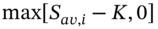
. European options are said to be path independent. On the other hand, it may be profitable to exercise an American option prior to expiration and hence this is a path-dependent option. Many exotic options are path dependent. For example, an Asian (average price) call option has a payoff which depends on the difference between the average price ![]() over the life of the option and the strike price. The Asian call payoff is
over the life of the option and the strike price. The Asian call payoff is ![]() and the value of
and the value of ![]() depends on the path taken by the stock price over the life of the option. Similarly, some options have a payoff which depend on the maximum or minimum value of the asset price over the life of the option – these are also path-dependent options.
depends on the path taken by the stock price over the life of the option. Similarly, some options have a payoff which depend on the maximum or minimum value of the asset price over the life of the option – these are also path-dependent options.
Some path-dependent options have closed-form solutions for the options price, as long as one assumes that the underlying asset price is monitored continuously. In practice, payoffs to path-dependent options usually depend on observations of the underlying asset price at discrete intervals (e.g. closing prices), and closed-form solutions may not be possible. Path-dependent options (with discrete monitoring) can often be priced using either the BOPM or MCS.
31.1 THREE-PERIOD BOPM
31.1.1 European Plain Vanilla Call Option
We use the ![]() period BOPM model. Assume the stock price can go up by 15%
period BOPM model. Assume the stock price can go up by 15% ![]() or down by 20%
or down by 20% ![]() each period.1 The initial stock price
each period.1 The initial stock price ![]() ,
, ![]() per period and the strike is
per period and the strike is ![]() . The risk-neutral probabilities for ‘up’ and ‘down’ moves are:
. The risk-neutral probabilities for ‘up’ and ‘down’ moves are:
where ![]() . The stock price tree is shown in Table 31.1:
. The stock price tree is shown in Table 31.1:
TABLE 31.1 Stock price tree
| Number of ups | ||||
| 3 | 152.09 | |||
| 2 | 132.25 | 105.80 | ||
| 1 | 115 | 92 | 73.60 | |
| 0 | 102 | 80 | 64 | 51.20 |
| Time | 0 | 1 | 2 | 3 |
To value a European option all we require are the four possible payoffs at maturity, which for a call option are max ![]() and for a put are max
and for a put are max ![]() . Using backward recursion through each node of the tree and risk neutral valuation RNV we obtain:
. Using backward recursion through each node of the tree and risk neutral valuation RNV we obtain:
There are ![]() alternative paths for the stock price through the 3-period tree (UUU, UUD, UDU, etc.). However, as the price of a European call (or put) depends only on the outcomes for the stock price at maturity of the option contract, we can simplify the above recursive calculation. So instead of looking at all (the nodes across all) the eight possible paths, we can simplify the computation by using the following binomial formula with
alternative paths for the stock price through the 3-period tree (UUU, UUD, UDU, etc.). However, as the price of a European call (or put) depends only on the outcomes for the stock price at maturity of the option contract, we can simplify the above recursive calculation. So instead of looking at all (the nodes across all) the eight possible paths, we can simplify the computation by using the following binomial formula with ![]() :
:
In the above formula the sum is only over k, the number of up moves, which has only four values, 0, 1, 2 and 3. This is a consequence of path independence since we are only concerned with the payoffs at ![]() . For example, for the paths with two ‘up moves’ that is UUD, UDU andDUU, they have the same value for
. For example, for the paths with two ‘up moves’ that is UUD, UDU andDUU, they have the same value for ![]() and these three outcomes are given by the term
and these three outcomes are given by the term  . Hence for these three paths we obtain the term ‘
![]() ’ in the above formula and we do not have to deal with each of the three paths separately.
’ in the above formula and we do not have to deal with each of the three paths separately.
Although it is more time consuming, we could also value the plain vanilla European call option as if it were path dependent. To do this we follow the stock price along each of the eight paths to get the eight possible payoffs to the call at ![]() . Each of these paths
. Each of these paths ![]() has a payoff equal to
has a payoff equal to ![]() . The risk neutral probability for each path is:
. The risk neutral probability for each path is:
where ![]() and
and ![]() . For example
. For example ![]() for the ‘three ups’ UUU-path would equal
for the ‘three ups’ UUU-path would equal ![]() while
while ![]() for each of the three paths with ‘two ups’ (i.e. UUD, DUU, and UDU) is
for each of the three paths with ‘two ups’ (i.e. UUD, DUU, and UDU) is ![]() . The call premium is then the present value of the expected payoffs along all eight paths using risk-neutral probabilities
. The call premium is then the present value of the expected payoffs along all eight paths using risk-neutral probabilities ![]() and discounting using the (continuously compounded) risk-free rate:
and discounting using the (continuously compounded) risk-free rate:
Of course this gives us the same answer as the binomial formula of Equation (31.2), which is computationally easier and quicker. Unfortunately, for path-dependent options we need to calculate the outcomes along every possible path through the lattice, since the payoffs depend on the particular path taken – this can be computationally burdensome – for ![]() periods (say).
periods (say).
31.2 ASIAN OPTIONS
Asian options have a payoff which is based on the average price over the life of the option. For example, an Asian (average price) call option has a payoff which depends on ![]() where
where ![]() is the average price over the life of the option.
is the average price over the life of the option.
An Asian average price currency option would be useful for a firm that wants to hedge the average level of its future receipts in foreign currency. The firm's monthly foreign currency receipts may fluctuate over the year so an Asian option is a cheap way to hedge, rather than using 12 vanilla calls with expiration dates in each of the months.
Average price Asian options have a payoff which depends on ![]() for a call and
for a call and ![]() for a put. There are also Asian average strike options and here the average price replaces the strike price, so the payoff for a call is
for a put. There are also Asian average strike options and here the average price replaces the strike price, so the payoff for a call is ![]() and for a put is
and for a put is ![]() . Since the underlying principles are similar, we do not discuss the Asian average strike option.
. Since the underlying principles are similar, we do not discuss the Asian average strike option.
The payoff from an Asian option (on a stock) may be based on the arithmetic or the geometric average of the underlying asset. For example, if the underlying price ![]() for one path in a 3-period tree is 100, 115, 132, 152 then the payoff to a call based on the arithmetic average would be
for one path in a 3-period tree is 100, 115, 132, 152 then the payoff to a call based on the arithmetic average would be ![]() and for the geometric average it would be
and for the geometric average it would be ![]() .2 The geometric average is always less than the arithmetic average (except when all values of
.2 The geometric average is always less than the arithmetic average (except when all values of ![]() are equal) and the difference between the two averages is greater, the greater the volatility of the price series.
are equal) and the difference between the two averages is greater, the greater the volatility of the price series.
Although analytic formulas (similar to Black–Scholes) for the price of an Asian option can be derived when the payoff is based on the geometric average, this is not the case for options based on the arithmetic average – which is unfortunate since the latter options are far more popular. It can be shown that (in a risk-neutral world) the geometric average of the asset price has the same probability distribution as the asset price itself, at maturity of the option, if the asset's expected growth rate is set equal to ![]() rather than the standard
rather than the standard ![]() and volatility is set at
and volatility is set at ![]() rather than
rather than ![]() . Hence we can price the geometric average option using the standard Black–Scholes formulas, with the above changes.
. Hence we can price the geometric average option using the standard Black–Scholes formulas, with the above changes.
How can we price an arithmetic average option? It can be shown that the distribution of the arithmetic average is approximately lognormal and therefore we can apply Black's equation for pricing futures-options, with the following changes. We calculate the first two moments (mean, ![]() and standard deviation,
and standard deviation, ![]() ) of the probability distribution of the arithmetic average (in a risk-neutral world) and fit a lognormal distribution to these moments. We then set
) of the probability distribution of the arithmetic average (in a risk-neutral world) and fit a lognormal distribution to these moments. We then set
and use Black's equation for futures options (see Chapter 25, Equations 25.15–25.18). Numerical methods such as the BOPM and Monte Carlo simulation are often used to price Asian options.
Consider an Asian (average price) call option on stock price ![]() , with
, with ![]() steps (using the same tree as above) which is reproduced in Table 31.2, for the eight possible paths for the stock price. The steps needed to price the Asian call using the BOPM are:
steps (using the same tree as above) which is reproduced in Table 31.2, for the eight possible paths for the stock price. The steps needed to price the Asian call using the BOPM are:
- Calculate average stock price
 at expiry, for each of the 8 possible paths
- Calculate the option payoff for each path:
- The risk-neutral probability for a particular path is
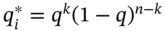
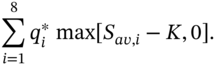
- Weight each of the eight outcomes for the payoff by their respective probabilities
 and sum them to give the risk-neutral expected payoff:
- The call premium is then the PV of the expected payoff discounted at the risk-free rate:
(31.5)
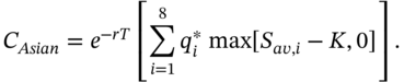
TABLE 31.2 Path in BOPM
| Path number | Path | Number of ups | Prob. | S(0) | S(1) | S(2) | S(3) | S (average) |
| 1 | UUU | 3 | 0.6297 | 100 | 115 | 132.25 | 152.09 | 124.83 |
| 2 | UUD | 2 | 0.1050 | 100 | 115 | 132.25 | 105.80 | 113.26 |
| 3 | UDU | 2 | 0.1050 | 100 | 115 | 92 | 105.80 | 103.20 |
| 4 | DUU | 2 | 0.1050 | 100 | 80 | 92 | 105.80 | 94.45 |
| 5 | UDD | 1 | 0.0175 | 100 | 115 | 92 | 73.60 | 95.15 |
| 6 | DUD | 1 | 0.0175 | 100 | 80 | 92 | 73.60 | 86.40 |
| 7 | DDU | 1 | 0.0175 | 100 | 80 | 64 | 73.60 | 79.40 |
| 8 | DDD | 0 | 0.0029 | 100 | 80 | 64 | 51.20 | 73.80 |
The eight final payoffs for the call option are shown in Table 31.3. The call premium for the Asian call option is ![]() . Similarly the price of an (average price) Asian put option is
. Similarly the price of an (average price) Asian put option is ![]() .
.
TABLE 31.3 Payoff to asian options
| Price call payoff | Price put payoff | Strike call payoff | Strike put payoff |
| 24.83 | 0 | 27.25 | 0 |
| 13.26 | 0 | 0 | 7.45 |
| 3.20 | 0 | 2.60 | 0 |
| 0 | 5.55 | 11.35 | 0 |
| 0 | 4.85 | 0 | 21.55 |
| 0 | 13.60 | 0 | 12.80 |
| 0 | 20.60 | 0 | 5.80 |
| 0 | 26.20 | 0 | 22.60 |
| 13.05 | 1.01 | 13.99 | 1.17 |
Notes:
Asian average price options payoffs are, for a call, max[S(average) – K,0] and for a put, max[K – S(average),0].
Asian average strike options payoffs are, for a call, max[S(3) – S(average),0] and for a put, max[S(average) – S(3),0]
The payoffs and option premia for Asian average strike options using the BOPM are calculated in a similar way and are shown in the last two columns of Table 31.3. The problem with using the binomial model to price the Asian option is that at least 50 steps are required to get an accurate measure of the option price and this requires evaluating 250 alternative paths! Even fast computers might not be quick enough to price the option in order to execute a deal.
The plain vanilla call costs more at ![]() than the Asian average call at
than the Asian average call at ![]() . Why? For a plain vanilla call, the call premium increases the higher is the volatility
. Why? For a plain vanilla call, the call premium increases the higher is the volatility ![]() of the underlying asset, S. The call premium for an Asian average price call (same underlying, strike, and maturity date) depends positively on the volatility of the average price,
of the underlying asset, S. The call premium for an Asian average price call (same underlying, strike, and maturity date) depends positively on the volatility of the average price, ![]() , where
, where ![]() is the number of values used to compute the average. If
is the number of values used to compute the average. If ![]() follows a Brownian motion and hence is identically and independently distributed (
follows a Brownian motion and hence is identically and independently distributed (![]() ) then
) then ![]() , which is smaller than
, which is smaller than ![]() . The Asian call premium that depends positively on
. The Asian call premium that depends positively on ![]() , will therefore be lower than the call premium on a plain vanilla call (which depends positively on
, will therefore be lower than the call premium on a plain vanilla call (which depends positively on ![]() ).
).
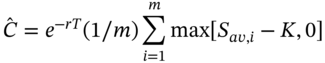
31.2.1 Monte Carlo Simulation (MCS)
An alternative and more efficient way to price an Asian option is to use MCS. Under risk-neutral valuation we ‘replace’ the real world growth rate of the stock ![]() with the risk-free rate
with the risk-free rate ![]() in the Brownian motion for the stock price. Assume the Asian option contract specifies that the underlying asset price
in the Brownian motion for the stock price. Assume the Asian option contract specifies that the underlying asset price ![]() will be observed each trading day when calculating the average price over the whole year and:
will be observed each trading day when calculating the average price over the whole year and:
As we have seen, MCS produces a series of alternative paths for the stock price using a discrete approximation to a Brownian motion. The payoff for an Asian (average price) call option for each run-i of the MCS over ![]() periods is:
periods is:
where ![]() is the average stock price over the 252 simulated trading days. The price of the Asian option is the PV of the payoffs (discounted at the risk-free rate) over all
is the average stock price over the 252 simulated trading days. The price of the Asian option is the PV of the payoffs (discounted at the risk-free rate) over all ![]() of the MCS:
of the MCS:
We need to choose ![]() large enough so that the error in estimating
large enough so that the error in estimating ![]() is acceptable (we can obtain a standard error for our estimate of
is acceptable (we can obtain a standard error for our estimate of ![]() as outlined in Chapter 26). Put in a more intuitive way, if we do
as outlined in Chapter 26). Put in a more intuitive way, if we do ![]() simulations then the calculated value for
simulations then the calculated value for ![]() should be ‘close to’ that found when using
should be ‘close to’ that found when using ![]() simulations.
simulations.
31.3 OTHER EXOTICS: LOOKBACKS, BARRIER, COMPOUND, AND CHOOSER
There is a virtually unlimited set of exotic options whose payoffs, time to maturity, strike price etc. can be ‘structured’ in the OTC market to suit the client's needs for either hedging or speculation. Needless to say the more ‘exotic’ the payoff structure, then generally speaking the more difficult they are to price and, often, numerical techniques are required. Below we briefly discuss some of the more common exotics.
31.3.1 Lookbacks (No-regrets) and Shout Options
Lookback options (on a stock) provide an investor with the opportunity to buy a stock at a potentially ‘low’ price (= long call option) or sell a stock at a potentially ‘high’ price (= long put option). For example, a lookback (European) call has the strike price set at expiration, at the lowest price ![]() of the stock during the life of the option, so the payoff is
of the stock during the life of the option, so the payoff is ![]() . Similarly, a lookback (European) put sets the strike price at expiration, equal to the highest price reached by the stock over the option's life, so the payoff is
. Similarly, a lookback (European) put sets the strike price at expiration, equal to the highest price reached by the stock over the option's life, so the payoff is ![]() .
.
These options are also referred to as no-regrets options since you would never regret not having exercised the option at an earlier date. The worst outcome possible with a lookback option is if it expires at-the-money (![]() ). There are also fixed strike lookbacks with payoffs for a call being
). There are also fixed strike lookbacks with payoffs for a call being ![]() and for a put,
and for a put, ![]() .
.
We have the complete set of paths for the stock price in the BOPM (see Table 31.2) and the associated risk neutral probabilities ![]() for each path. Hence, knowing the payoffs of the above lookbacks, it is easy to price them using the BOPM (or MCS). It should be obvious that European lookbacks have payoffs which are more favourable than ordinary European options and hence will have higher call and put premia.
for each path. Hence, knowing the payoffs of the above lookbacks, it is easy to price them using the BOPM (or MCS). It should be obvious that European lookbacks have payoffs which are more favourable than ordinary European options and hence will have higher call and put premia.
Shout options are European options that allow the holder to lock in a minimum payoff ![]() at one point in time
at one point in time ![]() during its life, but this payoff is not received until the expiration date,
during its life, but this payoff is not received until the expiration date, ![]() . For example, suppose the stock price rises so that a call option is currently in-the-money. With a shout option the holder, who may fear a future fall in stock prices, can ‘shout’ that the current payoff
. For example, suppose the stock price rises so that a call option is currently in-the-money. With a shout option the holder, who may fear a future fall in stock prices, can ‘shout’ that the current payoff ![]() , will be the minimum payoff at maturity. The payoff to the shout (call) option at
, will be the minimum payoff at maturity. The payoff to the shout (call) option at ![]() is max
is max ![]() .
.
But if the holder shouts at time ![]() , then the payoff to the shout option (at
, then the payoff to the shout option (at ![]() ) is
) is ![]() . Given the above payoff, the value of the shout option is the present value of
. Given the above payoff, the value of the shout option is the present value of ![]() (discounted from time T) plus the Black–Scholes value of a European call with a strike price
(discounted from time T) plus the Black–Scholes value of a European call with a strike price ![]() .
.
To price a shout call option using the BOPM we work backwards through the tree. At each node we calculate the (recursive) value if the holder does not shout and the value ![]() if the holder shouts and we take the greater of the two. This is similar to pricing a standard American option.
if the holder shouts and we take the greater of the two. This is similar to pricing a standard American option.
31.3.2 Barrier Options
Barrier options either ‘die’ or ‘come alive’ before expiration. For example, a knockout option may specify that if the stock price rises or falls to a ‘barrier level’, the option will terminate on that date, and hence cannot be exercised at a later date. If the option is terminated when the stock price falls to a lower barrier, we have a down-and-out option, while if it terminates when the price rises to a higher barrier, they are up-and-out-options. Option premia are paid ‘up front’ (at ![]() ).
).
Another variant of the barrier option is the up-and-in-option, whereby the option's ‘life’ does not begin until the stock price hits an upper barrier. The option premium is paid up front but the option cannot be exercised unless the stock price hits or crosses the upper barrier. Similarly a down-and-in-option is not ‘activated’ until the stock price hits (or crosses) the designated lower barrier.
31.3.2.1 Down-and-Out Put
Suppose you own a stock with current price ![]() and you buy a 1-year plain vanilla (European) put with strike
and you buy a 1-year plain vanilla (European) put with strike ![]() . If the stock price falls to
. If the stock price falls to ![]() at maturity, you obtain a cash payoff of
at maturity, you obtain a cash payoff of ![]() from the put, which implies your stock+put portfolio is worth $100 (the $9 cash plus the value of the stock $91) – you have provided a floor value for the stock of
from the put, which implies your stock+put portfolio is worth $100 (the $9 cash plus the value of the stock $91) – you have provided a floor value for the stock of ![]() .
.
Consider instead purchasing a 1-year down-and-in (European) put with ![]() and a ‘knock-in’ lower barrier set at
and a ‘knock-in’ lower barrier set at ![]() . If the stock price falls monotonically to say
. If the stock price falls monotonically to say ![]() at maturity, then your option will not have knocked-in and you will receive no payoff – this is a worse outcome than for the plain vanilla put. If at maturity
at maturity, then your option will not have knocked-in and you will receive no payoff – this is a worse outcome than for the plain vanilla put. If at maturity ![]() but sometime over the past year the stock price fell below
but sometime over the past year the stock price fell below ![]() , then your down-and-in put would have ‘come alive’ earlier and will now payoff
, then your down-and-in put would have ‘come alive’ earlier and will now payoff ![]() at maturity.
at maturity.
Hence for the down-and-in put to be worthwhile in providing a floor (at T), you must think that the stock price is going to be highly volatile over the next year, so it is likely that it would go through the lower barrier, ![]() , prior to expiration of the put. But why buy a down-and-in put when the vanilla put pays off in more states of the world? The answer is that a down-and-in put is cheaper than a vanilla put (with the same underlying, strike and maturity) since the down-and-in put doesn't come ‘alive’ until the lower barrier is hit. In other words you get what you pay for. With the down-and-in put, the payoff (at maturity) may be less than with the plain vanilla put, hence you pay less today for the down-and-in put.
, prior to expiration of the put. But why buy a down-and-in put when the vanilla put pays off in more states of the world? The answer is that a down-and-in put is cheaper than a vanilla put (with the same underlying, strike and maturity) since the down-and-in put doesn't come ‘alive’ until the lower barrier is hit. In other words you get what you pay for. With the down-and-in put, the payoff (at maturity) may be less than with the plain vanilla put, hence you pay less today for the down-and-in put.
31.3.2.2 Up-and-Out Put
Who might buy a European ‘up-and-out’ put? Consider a pension fund manager (Ms Long) who holds stocks that she wishes to ‘cash in’ after 1 year, or an oil producer (Mr Barrel) who will have barrels of oil ‘ready for sale’ in 1 year. Assume the stocks and oil are currently worth ![]() . In both cases suppose they think prices are highly unlikely to cross an upper barrier
. In both cases suppose they think prices are highly unlikely to cross an upper barrier ![]() over the next year. Also, assume they are both willing to ‘take a hit’ of a price fall of up to 10% (in oil or stock prices, but no more), by the year-end. They could protect their position by buying a 1-year out-of-the-money (OTM) vanilla put with a strike of
over the next year. Also, assume they are both willing to ‘take a hit’ of a price fall of up to 10% (in oil or stock prices, but no more), by the year-end. They could protect their position by buying a 1-year out-of-the-money (OTM) vanilla put with a strike of ![]() – but this might be expensive, given the volatility in stock or oil prices.
– but this might be expensive, given the volatility in stock or oil prices.
Instead, suppose Ms Long buys a European up-and-out put with a strike of ![]() and a ‘knock-out’ upper barrier of
and a ‘knock-out’ upper barrier of ![]() . If the stock price hits
. If the stock price hits ![]() on any day through the year, Ms Long loses her insurance (policy) on that day – that is, the put is now ‘dead’ and cannot be used to provide a floor of
on any day through the year, Ms Long loses her insurance (policy) on that day – that is, the put is now ‘dead’ and cannot be used to provide a floor of ![]() if prices fall below that level in 1 year's time. But if prices do not rise above
if prices fall below that level in 1 year's time. But if prices do not rise above ![]() on any day over the next year but they do fall below
on any day over the next year but they do fall below ![]() by the end of the year, the up-and-out put ‘remains alive’ and provides a floor of
by the end of the year, the up-and-out put ‘remains alive’ and provides a floor of ![]() . So there is more risk if you hold an up-and-out put rather than the vanilla put, but the up-and-out put costs you less.
. So there is more risk if you hold an up-and-out put rather than the vanilla put, but the up-and-out put costs you less.
31.3.2.3 Pricing Barrier Options
Pricing path-dependent barrier options using the BOPM or MCS is straightforward in principle. Again, consider the stock price lattice applied to down-and-out and down-and-in calls with the lower barrier set at ![]() , the upper barrier with
, the upper barrier with ![]() and the call is initially at-the-money,
and the call is initially at-the-money, ![]() (Table 31.4).
(Table 31.4).
TABLE 31.4 Barrier options
| Barrier | |||||||||||||
| 90 | 90 | 90 | 90 | 110 | 110 | 110 | 110 | ||||||
| Down-out and down-in options Payoffs | Up-out and up-in options Payoffs | ||||||||||||
| Path number | Path | S(0) | S(1) | S(2) | S(3) | Out call [1] | In call [2] | Out put [3] | In put [4] | Out call [5] | In call [6] | Out put [7] | In put [8] |
| 1 | UUU | 100 | 115.00 | 132.25 | 152.09 | 52.09 | Knock | 0 | Knock | Knock | 52.09 | Knock | 0 |
| 2 | UUD | 100 | 115.00 | 132.25 | 105.80 | 5.80 | Knock | 0 | Knock | Knock | 5.80 | Knock | 0 |
| 3 | UDU | 100 | 115.00 | 92.00 | 105.80 | 5.80 | Knock | 0 | Knock | Knock | 5.80 | Knock | 0 |
| 4 | DUU | 100 | 80.00 | 92.00 | 105.80 | Knock | 5.80 | Knock | 0 | 5.80 | Knock | 0 | Knock |
| 5 | UDD | 100 | 115.00 | 92.00 | 73.60 | 0 | Knock | 26.40 | Knock | Knock | 0 | Knock | 26.40 |
| 6 | DUD | 100 | 80.00 | 92.00 | 73.60 | Knock | 0 | Knock | 26.40 | 0 | Knock | 26.40 | Knock |
| 7 | DDU | 100 | 80.00 | 64.00 | 73.60 | Knock | 0 | Knock | 26.40 | 0 | Knock | 26.40 | Knock |
| 8 | DDD | 100 | 80.00 | 64.00 | 51.20 | Knock | 0 | Knock | 48.80 | 0 | Knock | 48.80 | Knock |
| Value of the option | 25.56 | 0.46 | 0.35 | 0.80 | 0.46 | 25.56 | 0.80 | 0.35 | |||||
Consider a down-and-out call. The payoff is ![]() as long as
as long as ![]() does not fall below
does not fall below ![]() . If any value of S along a particular path falls below
. If any value of S along a particular path falls below ![]() then the option knocks out (indicated by ‘knock’ in Table 31.4) and even if at expiration
then the option knocks out (indicated by ‘knock’ in Table 31.4) and even if at expiration ![]() , the payoff to this call is zero. Consider path number 4 (which is DUU) at
, the payoff to this call is zero. Consider path number 4 (which is DUU) at ![]() where
where ![]() . So even though along this path, at expiry
. So even though along this path, at expiry ![]() , nevertheless this call has a zero payoff, since it has already ‘died’. The payoffs for this call at
, nevertheless this call has a zero payoff, since it has already ‘died’. The payoffs for this call at ![]() , for all eight paths are shown in Table 31.4, column [1]. The call premium for the down-and-out call is simply the expected value of these eight payoffs (using risk-neutral probabilities
, for all eight paths are shown in Table 31.4, column [1]. The call premium for the down-and-out call is simply the expected value of these eight payoffs (using risk-neutral probabilities ![]() ), discounted at the risk-free rate, which gives
), discounted at the risk-free rate, which gives ![]() .
.
Notice that for ![]() , the sum of the option premia on the down-and-out call and the down-and-in call (i.e.
, the sum of the option premia on the down-and-out call and the down-and-in call (i.e. ![]() ), equals the premium for a plain vanilla European call,
), equals the premium for a plain vanilla European call, ![]() . This is because whenever the down-and-out call ‘dies’, the down-and-in call, ‘comes alive’, so if you hold both it is equivalent to holding a European vanilla call. This also demonstrates that the individual premia on the knock-out options are lower than the premia on the equivalent European vanilla options.
. This is because whenever the down-and-out call ‘dies’, the down-and-in call, ‘comes alive’, so if you hold both it is equivalent to holding a European vanilla call. This also demonstrates that the individual premia on the knock-out options are lower than the premia on the equivalent European vanilla options.
Take another example. If you want to insure a minimum value for a stock portfolio (![]() ) using a put with a strike of
) using a put with a strike of ![]() , you might consider buying an up-and-out put with an upper barrier at
, you might consider buying an up-and-out put with an upper barrier at ![]() which costs
which costs ![]() – this is cheaper than buying a vanilla put,
– this is cheaper than buying a vanilla put, ![]() (Table 31.4) – with the same strike and maturity date.
(Table 31.4) – with the same strike and maturity date.
Also, a speculator who expects a strong bull market but with little prospect of a steep fall in stock prices, might consider purchasing a down-and-out call because it costs less than (an equivalent) vanilla call. If the stock price over the life of the option does not fall below the lower barrier but a bull market also ensues, then the speculator can make a handsome profit.
Note that for barrier options, the nodes in the BOPM lattice would need to be aligned with the exact time the stock price is ‘checked’ against the barrier (e.g. each day at 4 p.m.). Table 31.4 also shows the outcomes and premia for some other European barrier options.
It should be clear from the above that MCS can easily be adapted to price barrier options. Consider a European knock-out call option. We simulate the stock price using a Brownian motion (under risk-neutrality) and if on a particular run of the Monte Carlo a barrier is crossed, then the payoff at expiration is set to zero even if ![]() If the barrier is not crossed, the payoff is
If the barrier is not crossed, the payoff is ![]() .
.
31.3.3 Compound Options
There are also options on options, known as compound options. Compound options have two strike prices and two exercise dates. For example, consider a call on a call. At ![]() the holder of the compound option can pay
the holder of the compound option can pay ![]() and take delivery of a call option, which gives her right to buy the underlying asset for
and take delivery of a call option, which gives her right to buy the underlying asset for ![]() at time
at time ![]() . The holder of the compound option will exercise at
. The holder of the compound option will exercise at ![]() only if the value of this option exceeds
only if the value of this option exceeds ![]() .
.
On 15 January an investor Ms Caution, decides that in 6 months' time (at ![]() ) she wants to buy a 2-year call option (on Apple stock) with a strike
) she wants to buy a 2-year call option (on Apple stock) with a strike ![]() . But on 15 January she is worried that by 15 June, the price of cash-market 2-year call options on Apple may have increased (above K1).
. But on 15 January she is worried that by 15 June, the price of cash-market 2-year call options on Apple may have increased (above K1).
On 15 January she therefore wants to fix the maximum price![]() she will pay on 15 June for ‘delivery’ of the 2-year call option on Apple, but she also wants to be able to take advantage of lower call premiums in the cash-market on 15 June, should this occur. Hence, on 15 January Ms Caution buys a ‘call on a call’, with a strike price
she will pay on 15 June for ‘delivery’ of the 2-year call option on Apple, but she also wants to be able to take advantage of lower call premiums in the cash-market on 15 June, should this occur. Hence, on 15 January Ms Caution buys a ‘call on a call’, with a strike price ![]() and pays (Morgan Stanley) the compound-option call premium of
and pays (Morgan Stanley) the compound-option call premium of ![]() (say).
(say).
On 15 June if the cash-market price of 2-year call options on Apple stock (with strike ![]() ) being offered by Goldman's (say) is
) being offered by Goldman's (say) is ![]() , Ms Caution will exercise her compound option with Morgan Stanley and take delivery of a 2-year call option (on Apple) at the low price
, Ms Caution will exercise her compound option with Morgan Stanley and take delivery of a 2-year call option (on Apple) at the low price ![]() . Alternatively, on 15 June if 2-year call options on Apple from Goldman's cost
. Alternatively, on 15 June if 2-year call options on Apple from Goldman's cost ![]() , she will not exercise the compound option with Morgan Stanley (and hence pay
, she will not exercise the compound option with Morgan Stanley (and hence pay ![]() ) and instead buys a cash-market 2-year call option on Apple stock from Goldman's, at the lower price of
) and instead buys a cash-market 2-year call option on Apple stock from Goldman's, at the lower price of ![]() . Hence a compound call option provides insurance against a future increase in call options prices. There are also puts-on-puts, puts-on-calls and calls-on-puts – but ‘enough already’. If we assume a GBM then European compound options have a complex closed-form solution that depends on integrals of the bivariate normal distribution (but we do not pursue that here).
. Hence a compound call option provides insurance against a future increase in call options prices. There are also puts-on-puts, puts-on-calls and calls-on-puts – but ‘enough already’. If we assume a GBM then European compound options have a complex closed-form solution that depends on integrals of the bivariate normal distribution (but we do not pursue that here).
31.3.4 Rainbow Options
Options can be structured to have a payoff based on the better or worse of two underlying assets and these are referred to as min-max, rainbow options or alternative options. For example, a rainbow call may pay off according to which of two underlying stocks (A or B) has the larger payoff at expiration.
31.3.5 Chooser Option
Sometimes an exotic option can be priced analytically because it can be decomposed into two ‘simpler options’ that do have exact pricing formulas. A chooser option or as-you-like-it option allows an investor to choose at a (known) specific point in time ![]() , whether the option is to be a call or a put. Once this choice has been made at
, whether the option is to be a call or a put. Once this choice has been made at ![]() , the option remains as either a call or a put (to its expiration date,
, the option remains as either a call or a put (to its expiration date, ![]() ). In a ‘standard chooser’, the call and put both have the same strike price and maturity and the choice has to be made at the prearranged time,
). In a ‘standard chooser’, the call and put both have the same strike price and maturity and the choice has to be made at the prearranged time, ![]() . ‘Complex choosers’ allow the holder to decide at any time before expiration whether to choose a call or put and the calls and puts may have different strikes and maturities. We only consider the standard chooser.
. ‘Complex choosers’ allow the holder to decide at any time before expiration whether to choose a call or put and the calls and puts may have different strikes and maturities. We only consider the standard chooser.
A chooser option is useful for speculating that there will either be a large rise (choose the call) or a large fall (choose the put) in the stock price between ![]() and
and ![]() . The prospective payoff at
. The prospective payoff at ![]() is therefore like a straddle but the chooser option has a lower premium. The reason for the lower premium is that a straddle always has a positive (gross) payoff, if either the call or the put is in-the-money at expiration (i.e.
is therefore like a straddle but the chooser option has a lower premium. The reason for the lower premium is that a straddle always has a positive (gross) payoff, if either the call or the put is in-the-money at expiration (i.e. ![]() or
or ![]() ). But with a ‘chooser’, after the choice is made at
). But with a ‘chooser’, after the choice is made at ![]() , there is a possibility that the chooser option will end up out-of-the-money (e.g. if you choose a call at
, there is a possibility that the chooser option will end up out-of-the-money (e.g. if you choose a call at ![]() and
and ![]() at expiration, then your chooser option has a zero payoff). The closer is the choice date to the maturity date of the options, the lower the probability of a wrong choice at
at expiration, then your chooser option has a zero payoff). The closer is the choice date to the maturity date of the options, the lower the probability of a wrong choice at ![]() and hence the chooser becomes more like a straddle.
and hence the chooser becomes more like a straddle.
An analytic solution for pricing a chooser option (on a stock which pays no dividends) is possible because it can be replicated using a long call and a long put – hence the price of the chooser is simply the sum of the ‘replication’ call and put premia. The analysis is a little involved and requires several steps.
First calculate whether the investor (Ms Dizzy) will choose a call or put. At ![]() , Ms Dizzy will choose the type of option which has the highest value. For example, she will choose a call if:
, Ms Dizzy will choose the type of option which has the highest value. For example, she will choose a call if:
Substituting for ![]() from put–call parity,
from put–call parity, ![]() (where the underlying asset has a constant dividend yield,
(where the underlying asset has a constant dividend yield, ![]() ) this implies:
) this implies:
Hence Ms Dizzy chooses the call at ![]() whenever the stock price at
whenever the stock price at ![]() exceeds
exceeds ![]() . Given the choice at
. Given the choice at ![]() , of either a call or put, the payoffs at maturity
, of either a call or put, the payoffs at maturity ![]() consequent on this choice are given in Table 31.5.
consequent on this choice are given in Table 31.5.
TABLE 31.5 Payoff to a chooser at T
| Payoff at T | ||
| Choice at t Chooser option |
|
|
| Call | 0 |
|
| Put |
|
0 |
To price the chooser option we need to consider a replication portfolio made up of ‘plain vanilla’ options that we can price using Black–Scholes. The price of the chooser option will then equal the price of this replication portfolio. The holder of the chooser at time ![]() will choose the more valuable of the two options:
will choose the more valuable of the two options:
Put–call parity at time ![]() :
:
Substituting in (31.11) for ![]() :
:
Rearranging (31.13):
The second term (in curly brackets) is the payoff from ![]() put options with strike
put options with strike ![]() which matures at
which matures at ![]() . From (31.14) we see that the chooser is equivalent to the following replication portfolio at
. From (31.14) we see that the chooser is equivalent to the following replication portfolio at ![]() :
:
- Long one European call with maturity
 and strike price
  plus
plus - Long
 European puts with maturity t and strike price
Hence using Black–Scholes the price of the chooser ![]() (at
(at ![]() ) is
) is
A straddle is a call and put with the same strike K and maturity ![]() , so it differs from a chooser because for the chooser, the put matures at
, so it differs from a chooser because for the chooser, the put matures at ![]() . If
. If ![]() then the chooser has the same call as the straddle but the chooser has a put with a lower strike and a shorter maturity – hence the chooser costs less than the straddle.
then the chooser has the same call as the straddle but the chooser has a put with a lower strike and a shorter maturity – hence the chooser costs less than the straddle.
31.4 SUMMARY
- Exotic (European) options have payoffs that are more complex than those from plain vanilla European options. Exotics are largely OTC instruments and their payoffs are structured to suit the needs of individual clients, in terms of maturity date, strike price, and different types of payoffs.
- Asian options have a payoff which is based on the average price of the underlying asset over the life of the option. They are useful when a corporate or an investor is paying or receiving periodic ‘cash flows’ (e.g. foreign currency).
- Barrier options either ‘die’ or ‘come alive’ before the expiration date, depending on whether the underlying asset price hits (or crosses) one or more barriers. These types of option cost less than the equivalent vanilla options (with the same underlying asset, strike price and time to maturity).
- Compound options are ‘options on options’. For example, buying a ‘call-on-a-call’ from Morgan Stanley sets the maximum price
 that you pay at
  for ‘delivery’ of a ‘second’ call option on Apple stock (say). This deliverable call option (on Apple stock) will have its own strike
  and maturity date
  . Like all call options, a compound call option also allows the holder to take advantage of lower cash-market call premia should this occur at
  . At expiration of the compound option at
  , if the premium for a cash-market call option on Apple stock (with strike
  and maturity date
  ), quoted by Goldman is
  then the compound option (with Morgan Stanley) is not exercised but instead the investor simply buys an identical cash-market call option from Goldman's at the lower price
  .
. - A chooser option allows the investor to choose at a specific point in time, whether the option is to be a call or a put.
- Lookback (European) options provide the investor with the opportunity to buy the stock (at maturity of the option) at the lowest price (lookback call) or to sell the stock at the highest price (lookback put) that has occurred over the life of the option.
- Many exotic (European) options are path dependent with a payoff at maturity that depends on all the possible paths taken by the underlying asset price and not just on the value of the underlying asset price on the expiration date of the option.
- For many exotic options closed-form solutions (like Black–Scholes) are not possible. Often, they are priced using numerical techniques such as binomial trees or Monte Carlo simulation or by solving a PDE by numerical methods (see Chapter 48).
EXERCISES
Question 1
Why might a US importer hedge using a long Asian (average price) call option on euros, with monthly averaging and maturity of one year?
Question 2
Explain the difference between path-dependent options and path-independent options and state why an American option is path dependent.
Question 3
Why might an investor holding stocks buy an up-and-out put. Intuitively, why is the price of an up-and-out put less than the price of a plain vanilla put?
Question 4
Why might a speculator buy an up-and-out put?
Question 5
Calculate the price of an (average price) Asian call option on a stock, using a two-period binomial model. Assume ![]() and the stock can go up 15% or down 10% per period. The risk-free rate
and the stock can go up 15% or down 10% per period. The risk-free rate ![]() per period and
per period and ![]() . Include the current stock price when determining the average price.
. Include the current stock price when determining the average price.
Question 6
Explain the steps used to price a knock-out call option with an upper barrier ![]() (which is greater than the current stock price,
(which is greater than the current stock price, ![]() ) using Monte Carlo simulation. The maturity of the option is
) using Monte Carlo simulation. The maturity of the option is ![]() ,
, ![]() ,
, ![]() p.a. (continuously compounded) and the barrier condition is monitored every 0.01 years (approximately every 2.5 trading days).
p.a. (continuously compounded) and the barrier condition is monitored every 0.01 years (approximately every 2.5 trading days).
Question 7
You are given the following information. Current stock price ![]() , the drift rate of stock price,
, the drift rate of stock price, ![]() p.a., risk-free rate
p.a., risk-free rate ![]() (continuously compounded), the volatility of stock returns
(continuously compounded), the volatility of stock returns ![]() p.a.,
p.a., ![]() and the time to maturity
and the time to maturity ![]() . Assume that
. Assume that ![]() (i.e. approximately 2.5 trading days) for the length of each timestep in the MCS.
(i.e. approximately 2.5 trading days) for the length of each timestep in the MCS.
Set out the steps you would take to price an Asian (average price) call option using Monte Carlo simulation. Assume ![]() is included in the averaging. (You can also set up the problem in Excel or some other convenient software.)
is included in the averaging. (You can also set up the problem in Excel or some other convenient software.)