CHAPTER 49
Equilibrium Models: Term Structure
Aims
- To show how bond prices and option prices can be derived from a model of the short-rate, using risk-neutral valuation.
- To investigate the properties of different time-series models of the short-rate.
- To demonstrate how continuous time models of the term structure can be used to price bonds and options on bonds.
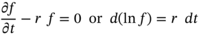
Black's model for pricing fixed income derivatives such as European options on bonds, on bond futures, as well as caps, floors, and swaptions, assumes the underlying variable is lognormal at expiration of the option. Black's model cannot price derivatives which depend on the evolution of interest rates through time – such as American style options, callable bonds and other path-dependent options.
The equilibrium yield curve approach assumes a specific continuous time stochastic process for the one period (short) rate. The parameters of this process are then estimated from historical data. Bond prices and fixed income derivatives prices can then be derived mathematically and these prices depend directly on the estimated parameters of the stochastic process for the short-rate. Hence, in the equilibrium approach the current term structure is an output from the short-rate model. (In contrast, in the no-arbitrage BOPM applied to fixed-income assets the current term structure is used as an input to calibrate the lattice for the short-rate.) The sequence of steps in the equilibrium model approach are:
- Choose a continuous time formulation for the short-rate and estimate the unknown parameters of this process, from historical data.
- Mathematically, derive the whole term structure from the chosen short-rate model.
- Use continuous-time mathematics to establish a PDE for the price of the fixed income derivative and solve the PDE to give a (closed-form) solution for the derivative's price (which then depends on the estimated parameters of the short-rate model).
It is worth noting at the outset that if the estimated time series model of the short-rate does not closely ‘fit’ the current observed behavior of interest rates, then the closed-form solution for the price of the derivative may not be accurate. However, it is not easy to empirically uncover what is the best statistical representation of the short-rate. This is a major practical drawback of this approach. However, we can still take a no-arbitrage approach, based on continuous time models for the short-rate, if we adapt these short-rate equations to fit today's term structure. This is sometimes possible by making the drift rate in the short-rate equation a function of time (e.g. Ho and Lee 1986 and Hull and White 1990). The mathematics of equilibrium models quickly becomes complex so we only present a heuristic overview of the approach.
49.1 RISK-NEUTRAL VALUATION
The instantaneous short-rate ![]() is the rate which applies over an infinitesimally short period of time (i.e.
is the rate which applies over an infinitesimally short period of time (i.e. ![]() to
to ![]() as
as ![]() ). Derivatives prices depend on the process for
). Derivatives prices depend on the process for ![]() in a risk-neutral world, so that if a derivative has a payoff
in a risk-neutral world, so that if a derivative has a payoff ![]() at time T then the current value
at time T then the current value ![]() of the derivative is:
of the derivative is:
where E* is the expected value in a risk-neutral world, ![]() is the average value of the short-rate (between t and T). We can use Equation 49.1 to price bonds and other fixed income assets (which depend on interest rates). For example, to value a zero-coupon bond which pays
is the average value of the short-rate (between t and T). We can use Equation 49.1 to price bonds and other fixed income assets (which depend on interest rates). For example, to value a zero-coupon bond which pays ![]() at
at ![]() , we have:
, we have:
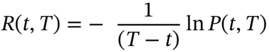
If ![]() is the observed continuously compounded interest rate on this ‘zero’ then it is known at time t, hence:
is the observed continuously compounded interest rate on this ‘zero’ then it is known at time t, hence:
It follows that:
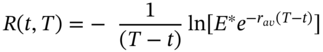
If we know the stochastic process for the short-rate ![]() in a risk-neutral world, then we can use (49.4b) to determine all the (continuously compounded) zero-coupon rates
in a risk-neutral world, then we can use (49.4b) to determine all the (continuously compounded) zero-coupon rates ![]() – that is, the complete term structure. First, we examine alternative plausible models for the instantaneous short-rate rate.
– that is, the complete term structure. First, we examine alternative plausible models for the instantaneous short-rate rate.
49.2 MODELS OF THE SHORT-RATE
The risk-neutral process for the instantaneous short-rate ![]() is usually an Ito process:
is usually an Ito process:
where ![]() is a Wiener process. We know today's short-rate,
is a Wiener process. We know today's short-rate, ![]() . Note that (49.5) is a ‘one-factor model’ since there is only one source of uncertainty,
. Note that (49.5) is a ‘one-factor model’ since there is only one source of uncertainty, ![]() . The crucial issue is how to choose a simplified tractable version of (49.5) which adequately represents the actual stochastic behaviour of the short-rate. Whether or not the short-rate exhibits (very slow) mean reversion or is non-stationary is a contested empirical issue (particularly since the advent of the literature on cointegration – see Cuthbertson and Nitzsche 2004). Hence, models of the short-rate both with and without mean reversion are used. Some alternatives are given below.
. The crucial issue is how to choose a simplified tractable version of (49.5) which adequately represents the actual stochastic behaviour of the short-rate. Whether or not the short-rate exhibits (very slow) mean reversion or is non-stationary is a contested empirical issue (particularly since the advent of the literature on cointegration – see Cuthbertson and Nitzsche 2004). Hence, models of the short-rate both with and without mean reversion are used. Some alternatives are given below.
49.2.1 Rendleman–Bartter (1980)
Here ![]() and
and ![]() in Equation (49.5) are assumed to be constant, hence
in Equation (49.5) are assumed to be constant, hence ![]() follows a GBM. But a GBM may give rise to negative values for the short-rate – so this model is somewhat unrealistic since observed nominal rates are hardly ever negative.1
follows a GBM. But a GBM may give rise to negative values for the short-rate – so this model is somewhat unrealistic since observed nominal rates are hardly ever negative.1
49.2.2 Ho–Lee (1986)
The Ho–Lee model has no mean-reversion but allows the drift rate to depend on ![]() :
:
The function ![]() is chosen so that the resulting forward rate curve fits the empirically observed term structure of forward rates. The function
is chosen so that the resulting forward rate curve fits the empirically observed term structure of forward rates. The function ![]() is the drift and represents the average direction in which the short-rate moves over time (and is independent of the level of
is the drift and represents the average direction in which the short-rate moves over time (and is independent of the level of ![]() so there is no mean-reversion). It can be shown that (approximately)
so there is no mean-reversion). It can be shown that (approximately) ![]() where
where ![]() and
and ![]() is the instantaneous forward rate. Hence the slope of the forward curve determines the direction the short-rate moves at time
is the instantaneous forward rate. Hence the slope of the forward curve determines the direction the short-rate moves at time ![]() .
.
With the Ho–Lee model, the price of zero-coupon bonds and European options on zero-coupon bonds can be determined analytically – see below. The Ho–Lee model can result in negative values for ![]() and in this respect the Hull–White model is an improvement.
and in this respect the Hull–White model is an improvement.
49.2.3 Hull–White (1990)
In contrast to the Ho–Lee model, the Hull–White model exhibits mean-reversion:
It is the term in square brackets that produces mean-reversion – the short-rate ![]() is pulled towards its equilibrium value
is pulled towards its equilibrium value ![]() . Thus if there were no stochastic shocks
. Thus if there were no stochastic shocks ![]() would move towards its long-run value of
would move towards its long-run value of ![]() , either from below if
, either from below if ![]() or from above if
or from above if ![]() . The parameter
. The parameter ![]() is determined by the initial term structure and it can be shown that:
is determined by the initial term structure and it can be shown that:
If we ignore the final term (which is small) then substituting ![]() in 49.7, the drift of the short-rate at time
in 49.7, the drift of the short-rate at time ![]() is
is ![]() . Hence, the path of the short-rate is determined by the slope of the initial forward rate curve, plus a mean-reverting component determined by the parameter
. Hence, the path of the short-rate is determined by the slope of the initial forward rate curve, plus a mean-reverting component determined by the parameter ![]() .
.
49.2.4 Black–Derman–Toy (1990)
This is the same as the Ho–Lee equation but with ![]() as the dependent variable and there is no mean-reversion:
as the dependent variable and there is no mean-reversion:
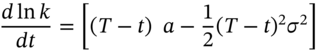
Using Ito's lemma the equation for ![]() is:
is:
49.2.5 Black–Karasinski (1991)
This approach takes the Black–Derman–Toy model and adds mean-reversion. If there are no stochastic shocks, ![]() approaches its equilibrium value
approaches its equilibrium value ![]() .
.
The advantage of this model (unlike Ho–Lee and Hull–White) is that interest rates cannot be negative, but its weakness is the difficulty in obtaining closed-form solutions for fixed income assets, even for simple cases such as the price of a zero-coupon bond.
49.2.6 Vasicek (1977)
This model has mean-reversion with a fixed value for the equilibrium level of interest rates of ![]() . The short-rate is assumed to be normally distributed and hence it is possible for
. The short-rate is assumed to be normally distributed and hence it is possible for ![]() to be negative:
to be negative:
49.2.7 Cox–Ingersoll–Ross (CIR 1985)
This has a fixed equilibrium value for the short-rate ![]() (as in the Vasicek model) and the standard deviation of the short-rate is proportional to
(as in the Vasicek model) and the standard deviation of the short-rate is proportional to ![]() . Hence as
. Hence as ![]() , the standard deviation approaches zero and short-rates are always non-negative. The risk-neutral process for
, the standard deviation approaches zero and short-rates are always non-negative. The risk-neutral process for ![]() is:
is:
In the ‘equilibrium model approach’, the parameters in the above equations are estimated from time series data. For example, in the CIR model, econometric estimates of ![]() and
and ![]() are required.
are required.
49.3 PRICING USING CONTINUOUS TIME MODELS
The above equations are one-factor models of the short-rate, as there is only one source of uncertainty. It is usually mathematically fairly difficult (although not impossible) to obtain a closed-form solution for a derivative security, when the underlying short-rate is governed by one of the above dynamic equations. We therefore consider a few simple cases which have analytic solutions but as the reader should note, these are largely for illustrative purposes only.
All the solutions take the short-rate equation as given and this leads to a PDE for the derivative's price. The solution to this PDE then gives the (closed-form) solution for the price of the derivative. The price of the derivative depends on the estimates of the parameters of the short-rate equation and the current value of the underlying asset (e.g. either the current short-rate or the zero coupon bond price), as well as the time to maturity ![]() of the derivative security. When closed-form solutions are not possible, the PDE can be solved for the derivatives price using numerical methods (e.g. finite-difference methods).
of the derivative security. When closed-form solutions are not possible, the PDE can be solved for the derivatives price using numerical methods (e.g. finite-difference methods).
49.3.1 Black–Scholes
Suppose we have a fixed income derivative security with price ![]() and the derivative has no payments until the terminal date
and the derivative has no payments until the terminal date ![]() (e.g. European style option). It can be shown that if
(e.g. European style option). It can be shown that if ![]() follows an Ito process (49.5), then the Black–Scholes PDE is (see Chapter 48) is:
follows an Ito process (49.5), then the Black–Scholes PDE is (see Chapter 48) is:
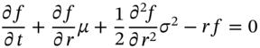
where![]() and
and ![]() may be functions of
may be functions of ![]() and
and ![]() . The payoff for the derivative at maturity
. The payoff for the derivative at maturity ![]() is assumed known – for example, for a call
is assumed known – for example, for a call ![]() where
where ![]() = price of the underlying asset.
= price of the underlying asset.
49.3.1.1 Solution 1: Zero-coupon Bond, Constant Short-rate
We price a zero-coupon bond using the Black–Scholes PDE, under the assumption of either constant or stochastic interest rates. A constant short-rate implies ![]() and
and ![]() , so (49.13) becomes:
, so (49.13) becomes:
This has a solution:
where ![]() is an arbitrary constant. The boundary condition is
is an arbitrary constant. The boundary condition is ![]() , the maturity value of the bond, which using (49.15) gives:
, the maturity value of the bond, which using (49.15) gives:
hence ![]() . Substituting in Equation (49.15) for
. Substituting in Equation (49.15) for ![]() gives:
gives:
Therefore the price of a zero coupon bond with face value ![]() and maturity
and maturity ![]() , when the interest rate is constant is:
, when the interest rate is constant is:
49.3.1.2 Solution 2: Zero-coupon Bond, Stochastic Interest Rates
Suppose the short-rate follows the Ho–Lee model:
where ![]() and
and ![]() are estimated parameters. First we assume a solution for the price of the zero coupon bond
are estimated parameters. First we assume a solution for the price of the zero coupon bond ![]() (with maturity value $1) of the form:
(with maturity value $1) of the form:
Hence: ![]() ,
, ![]() ,
, ![]()
Substitution in the Black–Scholes PDE, Equation (49.13), with ![]() gives:
gives:
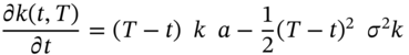
We now integrate (49.20b) over ![]() and incorporate the boundary condition,
and incorporate the boundary condition, ![]() to give:
to give:
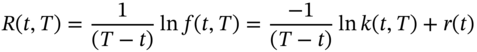
When (49.21) is substituted in (49.19) we have an explicit expression for the price ![]() of a zero-coupon bond which depends on the time to maturity
of a zero-coupon bond which depends on the time to maturity ![]() and the parameters of the short-rate process. The price of the zero-coupon bond will be consistent with no arbitrage along the yield curve (given the assumed Ho–Lee process for the short-rate rate). Substituting for
and the parameters of the short-rate process. The price of the zero-coupon bond will be consistent with no arbitrage along the yield curve (given the assumed Ho–Lee process for the short-rate rate). Substituting for ![]() from (49.19) in (49.4b):
from (49.19) in (49.4b):
Hence, in the Ho–Lee model an instantaneous change in the short-rate rate leads to an equal change in all long rates, that is, a parallel shift in the yield curve. This is a rather restrictive term structure model which could be made more flexible (and realistic) by using an alternative stochastic process for the short-rate rate, as illustrated below.
49.4 BOND PRICES AND DERIVATIVE PRICES
The Vasicek model incorporates mean reversion and it can be shown that the price of a zero-coupon bond is:
where ![]() and
and ![]() depend on the parameters of the short-rate equation:
depend on the parameters of the short-rate equation:
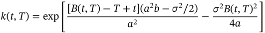
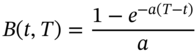
These expressions for ![]() and
and ![]() are more complex than those for the Ho–Lee model and they allow the yield curve (at time t) to be either (smoothly) upward or downward sloping or to exhibit a ‘humped shape’. The expression for long-rates is:
are more complex than those for the Ho–Lee model and they allow the yield curve (at time t) to be either (smoothly) upward or downward sloping or to exhibit a ‘humped shape’. The expression for long-rates is:

It is clear from the coefficient on ![]() in the above equation that when
in the above equation that when ![]() changes by 1%, long-rates do not all move by the same amount as the short-rate, so shifts in the yield curve are not constrained to be parallel.
changes by 1%, long-rates do not all move by the same amount as the short-rate, so shifts in the yield curve are not constrained to be parallel.
49.4.1 Call Option on a Zero-coupon Bond
It requires some complex continuous time mathematics to derive the closed-form solution for an interest rate derivative security based on the Vasicek, Ho–Lee, and Hull–White models. But Jamshidian (1989) has shown how a European call or put on a zero-coupon bond (or a coupon paying bond) can be priced. For example, for a call option on a zero-coupon bond that matures at time ![]() , the call premium has a closed-form solution of the form :
, the call premium has a closed-form solution of the form :
where Q = (principal) value of the bond, K = strike price of the bond, ![]() is the price of a deliverable bond with maturity value of $1 at any time
is the price of a deliverable bond with maturity value of $1 at any time ![]() (including
(including ![]() ),
), ![]() is the cumulative normal distribution and
is the cumulative normal distribution and ![]() is the maturity of the option. The terms
is the maturity of the option. The terms ![]() and
and ![]() are complex expressions which depend on
are complex expressions which depend on ![]() and the price of bonds of maturity
and the price of bonds of maturity ![]() and
and ![]() that is,
that is, ![]() and
and ![]() – as well as the parameters of the short-rate equation. The price of a put option is:
– as well as the parameters of the short-rate equation. The price of a put option is:
49.4.2 Option on Coupon Paying Bond
The CIR and Hull–White short-rate models can also be used to price European call and put options on zero-coupon bonds and can be adapted to price options on coupon paying bonds (Jamshidian 1989). For all one-factor models of the short-rate, zero-coupon bond prices of all maturities move up and down in unison as the short-rate changes. This allows European options on coupon-bonds to be expressed as the sum of the prices of options on zero-coupon bonds. A European swaption can be viewed as an option on a coupon paying bond and hence can be valued using one-factor models of the short-rate.
A further development is to assume the short-rate is influenced by two stochastic factors, for example by assuming that ![]() is also stochastic. Closed-form solutions for bond prices and interest rate derivatives can often be derived based on two-factor models (Longstaff-Schwartz 1992, Hull and White 1994).
is also stochastic. Closed-form solutions for bond prices and interest rate derivatives can often be derived based on two-factor models (Longstaff-Schwartz 1992, Hull and White 1994).
49.4.3 Hedging Using One-factor Models
Although one-factor models are usually accurate enough for pricing bonds and some European options, we cannot rely on accurate hedging of interest rate options, since one-factor models usually assume restrictive shifts in the yield curve, which are not realistic. The price of fixed-income derivatives can change substantially due to non-parallel shifts in the yield curve and due to changes in the term structure of volatility.2
As noted in an earlier chapter, there is not just one number for the delta, gamma, and vega of a fixed income derivative – because of different changes in spot rates and volatilities, along the yield curve. To put in place a hedge you first have to decide what type of shift in the yield curve you want to hedge against (e.g. a parallel shift or a twist in the yield curve). You then calculate the appropriate delta and gamma by changing each of the spot rates by the required amount and recalculating the derivatives (option) price under this new scenario – this is the ‘perturbation approach’ to obtaining the Greeks.
For example, the ‘5-year delta’ is the change in the value of your derivatives position for a small (1 bp) change in the 5-year spot yield. You can repeat this for spot rates at other maturities (e.g. 1 bp change in the 1-year spot rate) to give the derivatives portfolio deltas, for changes in several spot rates, along the yield curve. These changes in spot yields also imply changes in the forward curve and if the derivatives price depends on forward rates (e.g. caps and floors) these can also be incorporated in the calculation of delta.
Having obtained the deltas of your derivatives portfolio with respect to changes in several spot rates, you can then choose hedging instruments to offset these effects (e.g. using interest rate futures and other fixed-income options). The same procedure can be used to calculate the derivatives portfolio vega by changing volatilities along the yield curve, each by a small amount and calculating the change in the value of the derivative.
49.5 SUMMARY
- In the equilibrium model approach, the parameters of the chosen short-rate model are estimated. Continuous time mathematics is then used to derive a closed-form solution for bond prices and prices of fixed income derivatives (e.g. options on bonds, caps and floors etc.), which depend on the estimated parameters of the chosen short-rate equation.
- The main problem with the equilibrium approach is that small errors in estimating the short-rate parameters can lead to large errors in the price of the derivative security.
- Different models for the short-rate give different outcomes for the response of long-rates to changes in the short-rate – this is the ‘equilibrium’ term structure equation. Some short-rate models are restrictive, allowing only parallel shifts in the yield curve.
- When hedging, if we assume non-parallel shifts in the yield curve then we need to calculate the portfolio delta (or gamma or vega) of the fixed-income derivative with respect to specific changes in spot rates (or volatilities) along the yield curve – usually using a ‘perturbation approach’.
- The gamma and vega risk on a portfolio of fixed income options (on the same underlying) can be hedged using other fixed income options (e.g. caps, floors, options on T-bonds and on T-bond futures) with different maturities and strike prices. Finally, interest rate futures can be used to hedge any residual delta-risk with respect to changes in interest rates.
EXERCISES
Question 1
In the ‘equilibrium yield curve’ approach, explain why the estimated equation for the (one-period) short-rate is so important.
Question 2
In the equilibrium yield curve approach, derivatives are priced assuming a risk-neutral world. What is the key equation connecting a fixed income derivative's value today and the payoff to the derivative at maturity, T.
Question 3
Explain why you might not want to use a geometric Brownian motion, ![]() , as a realistic model of the short-rate.
, as a realistic model of the short-rate.
Question 4
Write down the Vasicek equation for the short-rate and explain how mean reversion is incorporated in the equation.
Question 5
What advantages does the Cox–Ingersoll–Ross (CIR) model for the short-rate have over the Vasicek model?
NOTES
- 1 In the low interest rate environment since 2010, some short-rates are negative (e.g. in Switzerland, Germany and Japan).
- 2 It may seem strange to assume changes in the yield curve that are not consistent with the short-rate equation used to price the derivative. But this is what we do when using the Black–Scholes model for pricing stock options and then vega hedging – the pricing model assumes a constant volatility but vega-hedging assumes volatility changes over time. In short, all models are approximations and their usefulness depends on the problem at hand and the size of any ensuing errors.