CHAPTER 39
Swaptions, Forward Swaps, and MBS
Aims
- To demonstrate how a payer swaption can be used to set an effective maximum swap rate that begins at expiration of the swaption but also allows the holder of the swaption to take advantage of lower (cash market) swap rates, should they occur in the future.
- To show how a long position in a forward swap locks in a known swap rate which will begin at expiration of the forward swap but the holder of the forward swap cannot take advantage of lower cash-market swap rates in the future should they occur.
- To analyse the use of various forms of mortgage-backed securities (MBS) and the interaction between interest rate changes, prepayment options, and the change in value of the MBS.
- To show how the Greeks can be used to hedge fixed income derivatives.
39.1 SWAPTIONS
Suppose you are thinking of taking out a 3-year pay-fixed (receive-float) vanilla interest rate swap in 2 years' time. You are worried that swap rates in 2 years' time will be high, implying you will pay a high fixed swap rate. If swap rates turn out to be low in 2 years' time then you will be happy to take advantage of this outcome. But you cannot know today what cash market swap rates will be in 2 years' time.
However, today, you would like to be able to fix the maximum swap rate you will pay in 2 years' time, whilst also being able to take advantage of low swap rates should they occur.
You can achieve this desired outcome if today you buy a 3-year payer swaption which expires in T = 2 years' time with a strike rate ![]() p.a., which is the agreed fixed swap rate. You have then insured that the maximum swap rate you will pay in the future is
p.a., which is the agreed fixed swap rate. You have then insured that the maximum swap rate you will pay in the future is ![]() but you can also take advantage of lower cash market swap rates should they occur, by not exercising the swaption and entering into a swap in the cash market in 2 years' time.
but you can also take advantage of lower cash market swap rates should they occur, by not exercising the swaption and entering into a swap in the cash market in 2 years' time.
The ‘underlying asset’ in the swaption contract is a 3-year cash market swap with an agreed payment frequency (tenor) and notional principal. At expiration, the buyer of the swaption may either ‘take delivery’ and enter into a cash market swap, or the swaption can be cash settled. The strike ![]() is the agreed swap rate in the swaption. The swaption premium will be paid up front.
is the agreed swap rate in the swaption. The swaption premium will be paid up front.
A swaption is an OTC option to enter into a cash market swap at the expiration date of the swaption, either as a fixed rate payer (at
) and floating rate receiver (i.e. payer swaption) or vice versa (i.e. a receiver swaption).
Suppose a US corporate thinks that it may need to borrow $10m at a floating rate from its correspondent bank (Citibank) for 3 years, beginning in 2 years' time. However, it wishes to swap the floating rate payments for fixed rate payments, thus transforming the loan to a fixed rate. The corporate therefore needs a ![]() swap (from Morgan Stanley, say), to pay fixed and receive floating beginning in 2 years' time and an agreement that the swap will last for a further 3 years (with annual payments).
swap (from Morgan Stanley, say), to pay fixed and receive floating beginning in 2 years' time and an agreement that the swap will last for a further 3 years (with annual payments).
Suppose the corporate thinks that interest rates will rise over the next 2 years and hence the cost of the fixed rate payments in the swap will be higher than at present. Rather than waiting for 2 years, the corporate can insure a maximum future swap rate by today purchasing (from Morgan Stanley) a 2-year European payer swaption, on a 3-year ‘pay-fixed, receive-floating’ swap, at a strike rate of ![]() (say). If cash market swap rates (quoted by JPMorgan, say) in 2 years' time are
(say). If cash market swap rates (quoted by JPMorgan, say) in 2 years' time are ![]() then the corporate will exercise the swaption and take delivery of a 3-year swap with a fixed swap rate equal to
then the corporate will exercise the swaption and take delivery of a 3-year swap with a fixed swap rate equal to ![]() , from Morgan Stanley.1 A payer swaption therefore places a ceiling on the fixed rate payable in a swap at
, from Morgan Stanley.1 A payer swaption therefore places a ceiling on the fixed rate payable in a swap at ![]() . However, if swap rates turn out to be
. However, if swap rates turn out to be ![]() in 2 years' time then the corporate would not exercise its payer swaption and would enter a cash market swap (with JPMorgan) at the current (low) swap rate of 9%.
in 2 years' time then the corporate would not exercise its payer swaption and would enter a cash market swap (with JPMorgan) at the current (low) swap rate of 9%.
39.1.1 Expiration of the Swaption
What is the payoff to a swaption if the cash market swap rate at expiration ![]() turns out to be
turns out to be ![]() The swap underlying the swaption is for delivery of a 3-year swap, with a notional principal Q = $10m and a strike swap rate of
The swap underlying the swaption is for delivery of a 3-year swap, with a notional principal Q = $10m and a strike swap rate of ![]() . Exercising the option allows one to enter into a swap to pay
. Exercising the option allows one to enter into a swap to pay ![]() fixed (and receive LIBOR). But at
fixed (and receive LIBOR). But at ![]() you could sell an otherwise identical 3-year swap in the cash market with fixed receipts at
you could sell an otherwise identical 3-year swap in the cash market with fixed receipts at ![]() (and pay LIBOR). The LIBOR payments in each swap cancel each other out.
(and pay LIBOR). The LIBOR payments in each swap cancel each other out.
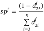
Hence the value (payoff) to the swaption at expiration is the present value of an annuity of ![]() , over 3 years (Figure 39.1):
, over 3 years (Figure 39.1):
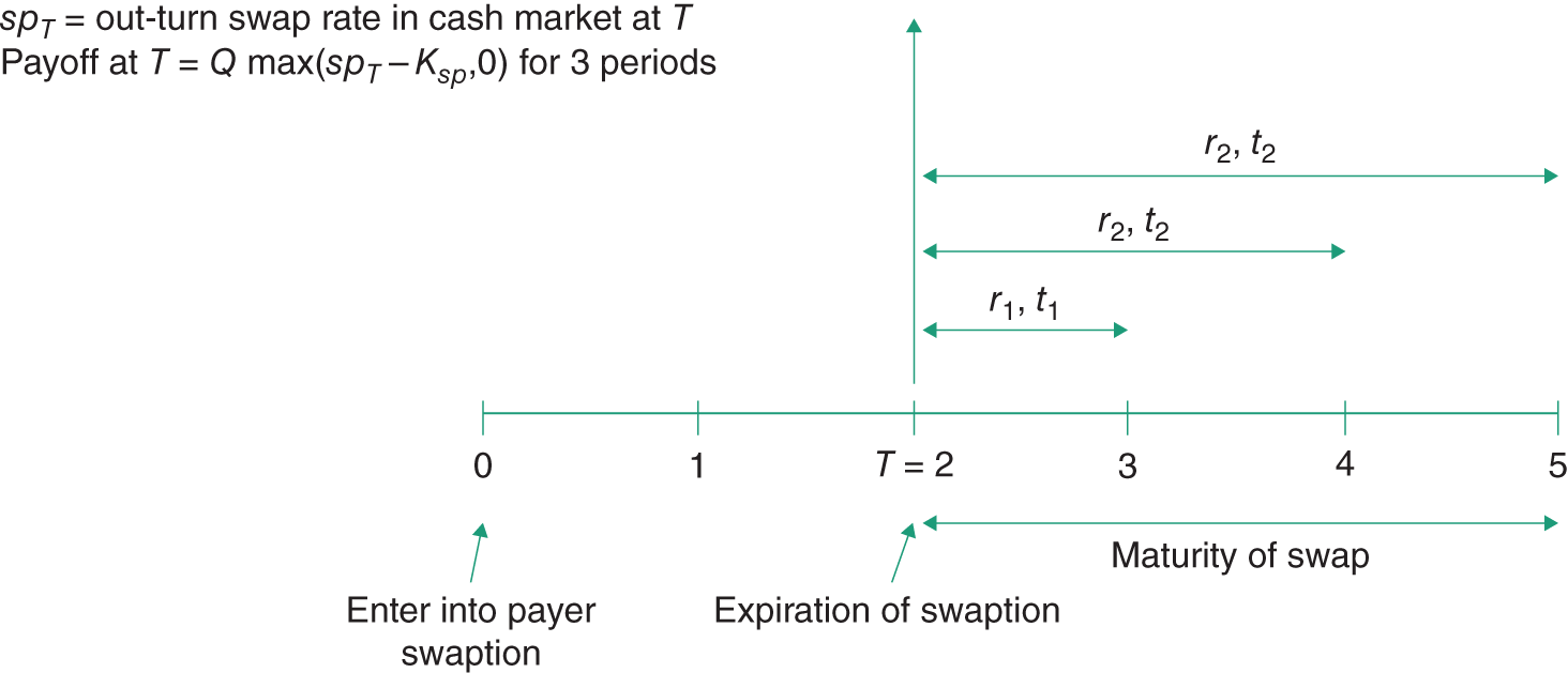
FIGURE 39.1 Payoff to European 3-year payer swaption
![]() = present value of an annuity of $1 paid at times
= present value of an annuity of $1 paid at times ![]() where
where ![]() using simple interest (or
using simple interest (or ![]() , continuously compounded rates).
, continuously compounded rates). ![]() is the out-turn spot rate at
is the out-turn spot rate at ![]() (the maturity date of the swaption (and ending i = 1, 2 or 3 years later).
(the maturity date of the swaption (and ending i = 1, 2 or 3 years later).
If the payer swaption is in-the-money, ![]() and is cash settled then at expiration
and is cash settled then at expiration ![]() is received by the holder of the swaption. Alternatively, if at expiration the underlying swap rate is
is received by the holder of the swaption. Alternatively, if at expiration the underlying swap rate is ![]() then the swaption would not be exercised but the corporate could then enter into a ‘new’ 3-year cash market swap at
then the swaption would not be exercised but the corporate could then enter into a ‘new’ 3-year cash market swap at ![]() , at the ‘low’ cash market swap rate of
, at the ‘low’ cash market swap rate of ![]() . Hence a payer swaption is an interest rate call where the payoff is the annuity value of
. Hence a payer swaption is an interest rate call where the payoff is the annuity value of ![]() , rather than simply a one-off payment of
, rather than simply a one-off payment of ![]() .
.
It should be obvious from the above that swaptions (either European or American) can also be used for speculation on the future value of the swap rate. You would buy a payer (receiver) swaption if you thought swap rates would rise (fall) in the future, relative to ![]() .
.
39.2 FORWARD SWAPS
A forward swap is a contract to enter into a swap at some future date, at a (forward) swap rate agreed today. Suppose you go long a 3-year forward swap with maturity ![]() years, notional principal
years, notional principal ![]() , annual tenor and a forward swap rate
, annual tenor and a forward swap rate ![]() . Then you have entered a contract today to ‘pay-fixed at
. Then you have entered a contract today to ‘pay-fixed at ![]() and receive-floating’, on a swap beginning in 2 years and lasting for a further 3 years.
and receive-floating’, on a swap beginning in 2 years and lasting for a further 3 years.
A long forward swap is a ‘pay-fixed, receive-floating’ swap that will commence in the future but at a forward swap rate
agreed today.
How do we price the forward swap at time ![]() ? (Figure 39.2).
? (Figure 39.2).
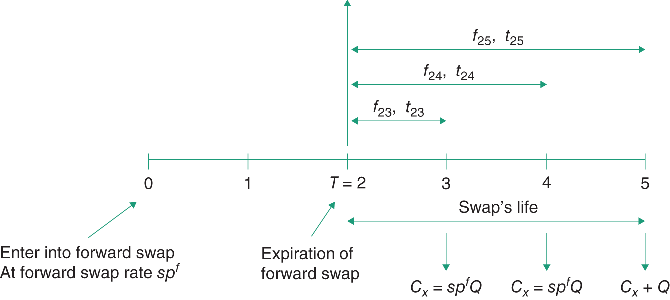
FIGURE 39.2 Two-year forward contract on a 3-year swap
39.2.1 Pricing a Forward Swap
The forward swap rate at ![]() is the fixed rate
is the fixed rate ![]() that makes the swap have zero expected value at
that makes the swap have zero expected value at ![]() (and therefore also at
(and therefore also at ![]() ). The floating leg of the swap (i.e. the FRN) is worth
). The floating leg of the swap (i.e. the FRN) is worth ![]() at
at ![]() . The fixed leg of the underlying swap has an annual coupon
. The fixed leg of the underlying swap has an annual coupon ![]() . The swap must have zero expected value at
. The swap must have zero expected value at ![]() :
:
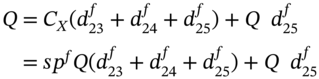
where ![]() and
and ![]() are the (simple) forward rates quoted at
are the (simple) forward rates quoted at ![]() which apply to periods from
which apply to periods from ![]() to
to ![]() . Hence the forward swap rate quoted today, for a swap with a maturity of
. Hence the forward swap rate quoted today, for a swap with a maturity of ![]() years, beginning in
years, beginning in ![]() years' time is:
years' time is:
The forward swap rate depends only on the individual forward rates (from year-2 onwards). The above formula is of the same form as that used earlier to determine today's cash market swap rate, ![]() , except that for the forward swap we use forward rates beginning at
, except that for the forward swap we use forward rates beginning at ![]() rather than spot interest rates beginning at
rather than spot interest rates beginning at ![]() .
.
39.2.2 Value of Forward Swap at Maturity
Assume ![]() for a 2-year forward swap on an underlying 3-year swap. Consider what happens at maturity
for a 2-year forward swap on an underlying 3-year swap. Consider what happens at maturity ![]() of the forward swap, if the forward swap is cash settled. Assume that at
of the forward swap, if the forward swap is cash settled. Assume that at ![]() the cash-market swap rate
the cash-market swap rate ![]() . The value at expiration
. The value at expiration![]() to the fixed rate payer (i.e. long forward swap) is the 3-year annuity value of the cash flow
to the fixed rate payer (i.e. long forward swap) is the 3-year annuity value of the cash flow ![]() :
:
where (using simple rates) the discount factors are ![]() and
and ![]()
![]() are the 1-year, 2-year and 3-year out-turn spot rates beginning at T = 2. Note that
are the 1-year, 2-year and 3-year out-turn spot rates beginning at T = 2. Note that ![]() are the actual spot rates (ex-post) known at
are the actual spot rates (ex-post) known at ![]() =2, which is now ‘the present’. If the out-turn cash market swap rate
=2, which is now ‘the present’. If the out-turn cash market swap rate ![]() = 12% >
= 12% > ![]() = 10% then the long receives cash of
= 10% then the long receives cash of ![]() at
at ![]() = 2, from the swap dealer. If the out-turn swap rate
= 2, from the swap dealer. If the out-turn swap rate ![]() = 8% <
= 8% < ![]() = 10% then the holder of the long forward swap pays out
= 10% then the holder of the long forward swap pays out ![]() to the swap dealer at
to the swap dealer at ![]() = 2.
= 2.
The difference between a forward swap and a swaption is that the latter allows the holder to benefit from any fall in swap rates, while also putting a known ceiling on the swap rate payable in the future. For this privilege you pay the swaption premium. In contrast, the forward swap ‘locks in’ a swap rate ![]() payable in the future and this implies you cannot take advantage of low swap rates should they occur – but by way of ‘compensation’, the forward swap does not require an up-front payment (we ignore margin payments).
payable in the future and this implies you cannot take advantage of low swap rates should they occur – but by way of ‘compensation’, the forward swap does not require an up-front payment (we ignore margin payments).
39.3 MORTGAGE-BACKED SECURITIES (MBS)
US financial institutions – primarily banks, savings and loan associations (S&Ls) and mortgage companies – issue fixed-rate mortgages with initial terms of between 15 and 30 years. However, these mortgages can be bundled up into a portfolio and sold to investors in the form of mortgaged-backed securities (MBS). This is securitisation – in the US and UK the MBS primary and secondary market is very large. The principal and interest payments of a MBS are often guaranteed by a government agency (e.g. in the US, the Government National Mortgage Association GNMA or ‘Ginnie Mae’). Securitisation can also be based on future receipts from other ‘assets’ such as car loans, credit cards, recording royalties, telephone charges, or many other types of loan repayments – as we see in Chapter 43.
39.3.1 Mortgage Pass-throughs and Strips
There are a wide variety of ways that MBS can be structured and then sold on to investors (i.e. mutual funds, pension funds, hedge funds, sovereign wealth funds, and wealthy endowment funds – like those held by Harvard and Yale Universities).
The simplest MBS are mortgage pass-throughs. Here, the investor (periodically) receives a proportion of the interest and principal payments on the underlying mortgages. In a ‘mortgage pass-through’, the initial value of the underlying mortgages ![]() held by an investor is equal to the present value of the fixed (coupon) mortgage payments of
held by an investor is equal to the present value of the fixed (coupon) mortgage payments of ![]() (per period) plus the present value of any repayments of principal. The discount rates used to calculate the present value are often risk-free yields, since many mortgage payments are guaranteed by institutions such as GNMA. Otherwise the discount rate is a risk-free rate plus a spread, to reflect the credit risk of the mortgagees.
(per period) plus the present value of any repayments of principal. The discount rates used to calculate the present value are often risk-free yields, since many mortgage payments are guaranteed by institutions such as GNMA. Otherwise the discount rate is a risk-free rate plus a spread, to reflect the credit risk of the mortgagees.
The pass-throughs are subject to considerable interest rate risk. Firstly, they are long maturity (high duration) ‘bonds’ and hence their (present) value (PV) rises (falls) when interest rates fall (rise) – this is a ‘pure interest rate effect’.
Secondly, the pass-throughs are subject to prepayment risk. If interest rates fall, then some home owners will want to pay off their existing fixed-rate mortgages and refinance at new lower rates. Hence, the holder of a pass-through may find prepayments increasing but she loses some of the future interest payments on the mortgages, which no longer need to be paid (as the mortgage has been paid off early). The change in value of a mortgage pass-through to investors is therefore complex depending on the interaction of the pure interest rate effect and prepayments. Conversely, if market interest rates rise, the pure interest rate effect will reduce the PV of the mortgage pass-through but mortgagees may extend the life of the mortgage.
Mortgage pass-throughs can be split into interest-only (IO) and principal only (PO) strips. The investor can buy a share of either the IO or the PO strip, or both.
An interest only (IO) strip entitles the investor to receive only interest payments from the portfolio of mortgages.
A principal only (PO) strip entitles the investor to receive only the payments of principal.
To illustrate what might happen to the change in value of a pass-through (PT) we consider the separate effects on the present value (PV) of IO and PO strips, and use the relationship ![]() .
.
When interest rates fall, the PV of any set of fixed interest payments will increase but any increase in prepayments will reduce the PV of an IO strip, as the prepayments imply that many future interest payments are now not required to be paid. The net effect is usually a fall in the value of IO strips, after a fall in interest rates, because of a high level of prepayments by mortgagees.
If interest rates rise, the PV of an IO strip will fall due to the pure interest rate effect but this may be offset by a lengthening of the life of the mortgage and hence the interest payments, so the overall effect may be an increase in value of the IO strip.
We can illustrate the effect of changes in interest rates on IO and PO strips and pass-throughs, by considering the following ‘stylised’ portfolio of mortgages.
- Value of initial mortgage
 = $100,000
 - Life of initial mortgage
 = 10 years
 - Fixed rate agreed for mortgage repayments
 = 10% p.a.
The fixed amount paid by the mortgagees ![]() p.a., must ensure that the present value of all the payments
p.a., must ensure that the present value of all the payments ![]() equals the current value of the mortgage advance,
equals the current value of the mortgage advance, ![]() . Hence, the required fixed annual mortgage payment
. Hence, the required fixed annual mortgage payment ![]() is the solution to:
is the solution to:
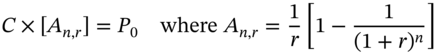
![]() is the PV of an annuity (of $1 payable) over n-years, given the current (n-year) interest rate (yield),
is the PV of an annuity (of $1 payable) over n-years, given the current (n-year) interest rate (yield), ![]() . Solving the above equation gives
. Solving the above equation gives ![]() = $16,275 p.a. In the first year, the interest accruing on the loan is
= $16,275 p.a. In the first year, the interest accruing on the loan is ![]() = $10,000 =
= $10,000 = ![]() which implies that (
which implies that (![]() ) is $6,275 can be used to reduce the initial principal, leaving an outstanding balance at the end of year-1,
) is $6,275 can be used to reduce the initial principal, leaving an outstanding balance at the end of year-1, ![]() = $100,000 – $6,275. For each succeeding year:
= $100,000 – $6,275. For each succeeding year:
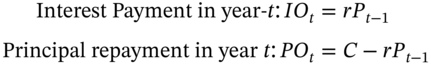
![]() is calculated recursively:
is calculated recursively:
An investor (Mr Strip) who purchases an IO strip today, will be willing to pay the present value of the future mortgage interest payments. Suppose ![]() p.a. is the current annual yield2 and we also (somewhat arbitrarily) assume that with
p.a. is the current annual yield2 and we also (somewhat arbitrarily) assume that with ![]() , the average life of the mortgages in the securitised mortgage pool is 7 years because of early prepayments by some homeowners. The
, the average life of the mortgages in the securitised mortgage pool is 7 years because of early prepayments by some homeowners. The ![]() of these interest payments (Table 39.1, column 4) is:
of these interest payments (Table 39.1, column 4) is:
TABLE 39.1 Mortgage-backed securities (MBS)
| Years | Loan outstanding | Fixed payments | Interest accrual | Repayment of principal | Loan outstanding after payments | NPV | ||
| IO | PO | |||||||
| 1 | 100,000 | 16,274.54 | 10,000 | 6,274.54 | 93,725.46 | |||
| 2 | 93,725.46 | 16,274.54 | 9,372.55 | 6,901.99 | 86,823.47 | NPV(7%, 2 years) | £17,532.14 | £87,727.50 |
| 3 | 86,823.47 | 16,274.54 | 8,682.35 | 7,592.19 | 79,231.27 | |||
| 4 | 79,231.27 | 16,274.54 | 7,923.13 | 8,351.41 | 70,879.86 | |||
| 5 | 70,879.86 | 16,274.54 | 7,087.99 | 9,186.55 | 61,693.31 | |||
| 6 | 61,693.31 | 16,274.54 | 6,169.33 | 10,105.21 | 51,588.10 | |||
| 7 | 51,588.10 | 16,274.54 | 5,158.81 | 11,115.73 | 40,472.37 | NPV(7%, 7 years) NPV(8%, 7 years) NPV(9%, 7 years) |
£43,041.21 £41,732.57 £40,487.63 |
£69,871.16 £66,613.94 £63,561.14 |
| 8 | 40,472.37 | 16,274.54 | 4,047.24 | 12,227.30 | 28,245.07 | |||
| 9 | 28,245.07 | 16,274.54 | 2,824.51 | 13,450.03 | 14,795.04 | |||
| 10 | 14,795.04 | 16,274.54 | 1,479.50 | 14,795.04 | 0 | NPV(9%, 10 years) | £44,444.24 | £60,000.19 |
where using compound rates, ![]() . Similarly, an investor (Mr Principal) who purchases the principal only strip will be willing to pay the present value of the repayments of principal (Table 39.1, column 5) up to the end of year-7, plus the remaining principal
. Similarly, an investor (Mr Principal) who purchases the principal only strip will be willing to pay the present value of the repayments of principal (Table 39.1, column 5) up to the end of year-7, plus the remaining principal ![]() after early redemption by some mortgagees, hence:
after early redemption by some mortgagees, hence:
The value of a ‘pass-through’ is simply the sum of the IO and PO strips, which is:
An investor in a mortgage pass-through has a claim on a set of coupon and principal payments. The reason MBS are derivative securities is that an investor in a MBS has implicitly written (sold) an American put option because the mortgagee has the right to redeem the mortgage. The strike price in the embedded put option is equal to the outstanding principal of the mortgage. Conversely, householders paying the mortgage have a long put which they will be more likely to exercise (i.e. remortgage), the lower are market interest rates in the future.
Let us consider what happens to the value of the IO and PO strips when interest rates change. We shall see that changes in value for the IO and PO strips depends crucially on how interest rates affect whether the prepayment option is exercised.
39.3.2 Interest Only Strips
If ![]() falls to 7% and the prepayment date remains at the end of year-7 then
falls to 7% and the prepayment date remains at the end of year-7 then ![]() increases from $41,733 to $43,041 (i.e. pure interest rate effect). But if
increases from $41,733 to $43,041 (i.e. pure interest rate effect). But if ![]() falls to 7% and this moves the average prepayment date to the end of year-2,3 then today the IO strip is only worth:
falls to 7% and this moves the average prepayment date to the end of year-2,3 then today the IO strip is only worth:
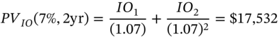
So although the fall in ![]() from 8% to 7% raises the PV of each interest receipt, the number of interest payments has dropped from seven to two. Hence there is a substantial fall in
from 8% to 7% raises the PV of each interest receipt, the number of interest payments has dropped from seven to two. Hence there is a substantial fall in ![]() from $41,733 to $17,532, a fall of 60%.
from $41,733 to $17,532, a fall of 60%.
Now suppose that y increases from 8% to 9%. If the average life of the mortgages remains at 7 years, then ![]() will fall from $41,733 to $40,488. However, if the life of the average (fixed interest) mortgage is extended to 10 years, then there is an increase in
will fall from $41,733 to $40,488. However, if the life of the average (fixed interest) mortgage is extended to 10 years, then there is an increase in ![]() from $41,733 to $44,444 (6.5%), because of the increased number of interest payments (even though these are discounted at a higher rate). Hence, the change in value of
from $41,733 to $44,444 (6.5%), because of the increased number of interest payments (even though these are discounted at a higher rate). Hence, the change in value of ![]() depends crucially on the interaction between the change in
depends crucially on the interaction between the change in ![]() (‘pure interest rate effect’) and the change in the average prepayment period (i.e. whether the prepayment option is exercised by the homeowner).
(‘pure interest rate effect’) and the change in the average prepayment period (i.e. whether the prepayment option is exercised by the homeowner).
39.3.3 Principal Only Strips
There will be some early prepayments of principal simply because people move house for a whole variety of reasons (e.g. arrival of children, changing jobs etc.). But here we only concentrate on the interaction between interest rates and the prepayment option.
Suppose ![]() falls from 8% to 7% or rises from 8% to 9%, with no change in the 7-year maturity of the underlying mortgages. Clearly, after an interest rate fall (rise)
falls from 8% to 7% or rises from 8% to 9%, with no change in the 7-year maturity of the underlying mortgages. Clearly, after an interest rate fall (rise) ![]() rises (falls), ceteris paribus. However, if the fall in
rises (falls), ceteris paribus. However, if the fall in ![]() from 8% to 7% brings the average prepayment date to the end of year-2, then:
from 8% to 7% brings the average prepayment date to the end of year-2, then:
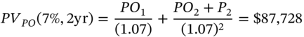
where ![]() (Table 39.1, column 6, row 2) is the ‘large’ prepayment of the remaining principal on the mortgages at the end of year-2. Hence
(Table 39.1, column 6, row 2) is the ‘large’ prepayment of the remaining principal on the mortgages at the end of year-2. Hence ![]() increases substantially from
increases substantially from ![]() = $66,614 to
= $66,614 to ![]() = $87,728, that is, an increase of 31.7%.
= $87,728, that is, an increase of 31.7%.
Alternatively, if interest rates rise immediately from 8% to 9% and this pushes the prepayment date out to year-10, then ![]() falls substantially from
falls substantially from ![]() = $66,614 to
= $66,614 to ![]() = $60,000, that is, a fall of 9.9%.
= $60,000, that is, a fall of 9.9%.
From Table 39.1 we can calculate the PV of the mortgage pass-through using ![]() for our three cases:
for our three cases:
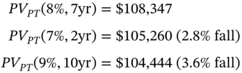
Hence here, the value of the mortgage ‘pass-through’ is less sensitive to interest rate changes and consequent changes in the schedule of prepayments by homeowners, than are IO and PO strips, taken separately. The value of IO and PO strips are very sensitive to the complex interaction between changes in interest rates and any prepayments by homeowners, which also depend on the characteristics of the cohort of mortgage borrowers – such as age, marital status, number of children, geography, income, state of the (local) economy etc. Hence it is difficult to value and predict changes in IO and PO strips. While they (often) carry a government credit guarantee, there is no guarantee that their market value will remain unchanged and hence they are far from being ‘safe investments’ – as the events of the crash of 2008–9 illustrated.
39.4 HEDGING FIXED INCOME DERIVATIVES
The price of fixed income derivatives, such as options on T-bond futures or caps and floors, can change substantially due to non-parallel shifts in the yield curve or changes in the term structure of volatility. There is therefore not just ‘one number’ for the delta, gamma, and vega of a fixed income derivative – for example, you can have a delta for a cap with respect to the 3-month interest rate, the 6-month rate etc. Once you have calculated the type of shift in the yield curve you want to hedge against (e.g. for a parallel shift or a twist in the yield curve) then you can calculate the appropriate delta and gamma by recalculating the option price under this new interest rate scenario, using an option pricing formula such as Black's model – this is the ‘perturbation approach’.
Suppose we want to calculate the delta of an option on a fixed income asset (e.g. option on a T-bond or option on Eurodollar futures). The delta is defined as the change in the option price due to a (small) change in spot yields (i.e. the ‘zero curve’). Possible alternative ways of modelling and simulating changes in interest rates along the yield curve are:
- Calculate the change in the option price due to a parallel shift in all spot yields of 1 bp – this is sometimes referred to as a PV01, DV01, or PVBP – that is, the ‘present value’ or ‘duration value’ of a 1 bp (0.01%) parallel shift.
- Divide the zero curve (or forward curve) into a number of ‘maturity buckets’ and calculate the change in the option's price for a 1 bp change in one of these time buckets (e.g. for 0–3 month rates), holding the rest of the yield curve unchanged. Or alternatively calculate the change in the options price for a 2 bp change in one time bucket (e.g. 0–3 month rates) and a 1 bp change in another time bucket (e.g. 4–6 month rates) – to mimic a twist in the yield curve.
- Use a principal components analysis to decompose all spot rate changes across the yield curve into say the ‘first 3 principal components’. Then calculate a delta for each of these three principal components (PC). The delta of the first-PC represents an (approximate) parallel shift in the yield curve, the delta for the second-PC represents a twist in the curve and the third-PC often can be interpreted as a possible ‘bowing’ of the yield curve.
- Calculate the change in the option's price due to small changes in all the ‘yields’ that have been used to construct the zero curve. The easiest way to think of this is that all spot rates are changed by different amounts based on a trader's view of likely ‘shifts’ along the yield curve – this is like the ‘bucket’ case but with many more ‘buckets’.
- A slightly more complex variant is to use the actual rates used to construct the yield curve. If the short end of the curve has been derived using yields based on zero-coupon bonds (bills) then these yields would be changed by a small amount. If the long end of the curve is constructed from spot yields derived from swap rates, then swap rates would be changed by a small amount.
Once we have our new spot rates we can calculate a new price for the (fixed income) option using an appropriate pricing formula (e.g. Black's model) and hence calculate the option's (overall) delta.
Calculating gamma is even more involved. Suppose there are five different spot rates ![]() used to construct the zero curve and to price the option (e.g. swaption). Then there are at least five different gammas with respect to changes in these five different spot rates, which influence the change in the option's price
used to construct the zero curve and to price the option (e.g. swaption). Then there are at least five different gammas with respect to changes in these five different spot rates, which influence the change in the option's price ![]() . (This assumes we ignore cross product terms
. (This assumes we ignore cross product terms ![]() in the Taylor series expansion of
in the Taylor series expansion of ![]() .) But once we have made our specific choice of a specific shift in the yield curve (e.g. parallel shift), the calculation of specific gammas using the perturbation method is straightforward, in principle.
.) But once we have made our specific choice of a specific shift in the yield curve (e.g. parallel shift), the calculation of specific gammas using the perturbation method is straightforward, in principle.
The same procedure can be used to calculate vega by changing the volatility (of interest rates) by a small amount and calculating the change in the option premium. If the option premium depends on the volatility of interest rates at different horizons then when calculating the option's vega we can either assume an equal change in all volatilities or we can change volatilities by different amounts at different maturities (e.g. change the volatility of 3-month interest rates by a different amount than you change the volatility of 6-month rates).
39.4.1 Hedging Interest Rate Options and Swaps
Suppose a bank acts as a swap dealer and also buys and sells interest rate options such as caps and floors (to corporates and other banks). A long position in an interest rate cap increases in value as interest rates increase – it has a positive delta. So if a bank sells a cap (to a corporate) and interest rates rise, the bank loses – a short cap has a negative delta.
A cap is a series of caplets on an agreed notional principal. For simplicity assume MegaBank on 15 June 2019 holds a cap which consists of three caplets with maturity dates of September-2019, March-2020 and September-2020. Each caplet has a known price (on 15 June 2019). If we assume a 1 bp increase in interest rates (over 1 day say) then we can work out the change in value (over 1 day) of each caplet and hence of the cap itself. The cap will also have a gamma (with respect to interest rates) and a vega (with respect to the volatility of interest rates, ![]() ).4
).4
Assume MegaBank has positions in swaps and caps – how does the bank hedge these positions? We proceed as we did when hedging a portfolio of stock options (see Chapter 18) but here it is changes in interest rates and the volatility of interest rates that cause changes in the value of MegaBank's caps or swaps. We can easily calculate the total gamma and vega of MegaBank's ‘swaps plus cap’ portfolio. (The vega only arises from the caps, the vega of a swap is zero.)
Our first hedging method for MegaBank's ‘swaps plus cap’ can be sequential because we choose first to hedge with an interest rate option-X and then with a fixed income asset with a zero vega (e.g. a T-bond, which has non-zero gamma and delta but a zero vega). We first use option-X to hedge the vega, then we hedge the gamma and finally the delta.
First, we use an interest rate option-X (e.g. cap with a different strike or expiration date) to offset the vega of MegaBank's current cap position – so we are now vega neutral. This will lead to a new portfolio gamma, since option-X has a non-zero gamma. We can offset this new portfolio gamma by buying or selling T-bonds or FRAs (which have non-zero gammas). The important point is that achieving a gamma-neutral portfolio using T-bonds does not upset our newly acquired vega neutral position – as T-bonds have zero vegas.
However, including bonds in our hedge portfolio to achieve gamma neutrality, will alter the delta of our portfolio, which we now recalculate. Finally, we offset this remaining portfolio delta by using Eurodollar futures (which have zero gamma and vega). We are then vega, gamma, and delta neutral and we have been able to hedge sequentially – first with option-X (vega neutral), then with bonds (gamma neutral) and finally with Eurodollar futures (to achieve delta neutrality).
Our second hedging method uses two interest rate options (e.g. a mixture of caps or bond options or bond futures options). This hedge cannot be done sequentially because the two options both have non-zero gammas and non-zero vegas. To hedge MegaBank's ‘swaps+caps’ position we first use two other interest rate options X and Y (e.g. caps with different strikes and expiration dates) to simultaneously hedge the gamma and vega of our initial position. (This was done for stock options in Chapter 18.) MegaBank's portfolio now consists of ‘swaps+caps+options-X+options-Y’ and has a portfolio gamma and vega that are both zero. But MegaBank, by adding the two options X and Y, has changed the delta of its initial ‘swap+caps’ portfolio, so it now recalculates its new portfolio delta. MegaBank then ‘neutralises’ this new portfolio delta by taking offsetting positions in Eurodollar futures – which does not affect MegaBank's existing vega-gamma neutral position because Eurodollar futures contracts have zero vega and gamma.
39.5 SUMMARY
- A payer swaption is an option on a swap. If you hold a payer swaption with a strike
 , you have effectively placed an upper limit of
  on the fixed rate payable in a swap (which will start at the expiration date of the swaption contract). However, you can also take advantage of low cash market swap rates in the future by not exercising the swaption at maturity, if the out-turn swap rate
  is below
  and instead you purchase a cash market swap at the low swap rate,
  .
. - A forward swap can be used by a corporate to ‘lock in’ a known swap rate that will begin at a specific time in the future. However, the corporate cannot then benefit from lower swap rates in the future should these occur.
- One of the largest and most active fixed income markets is for various forms of mortgage-backed securities (MBS). It is the prepayment possibility in these portfolios of mortgages that give them their ‘embedded option’ characteristics. The market value of mortgage pass-throughs, interest only and principal only strips are very sensitive to the interaction between changes in interest rates and the decision to prepay the principal early (or to extend the life of the mortgage).
- Calculating the Greeks for fixed income derivatives can be done by the perturbation method. For example, change the input (e.g. spot yields) by a small amount and recalculate the new option price (e.g. using Black's model or the BOPM) – this gives the option's delta for this specific set of spot rate changes. Other Greeks can be calculated in a similar way.
- A portfolio of options on fixed income assets (e.g. caps and floors) can be vega-hedged and gamma-hedged using other fixed income options (e.g. caps and floors with different strike prices and expiration dates) and finally delta-hedged using Eurodollar futures contracts.
EXERCISES
Question 1
A corporate treasurer has to borrow $10m in 2 years' time, at 360-day LIBOR, for a further 2 years. She decides to take out a forward swap, to receive-LIBOR and pay-fixed, with tenor 1 year. The swap will begin in 2 years.
Current forward rates (continuously compounded) are ![]() ,
, ![]() ,
, ![]() ,
, ![]() ,
, ![]() ,
, ![]() . Calculate and explain how the forward swap rate is determined.
. Calculate and explain how the forward swap rate is determined.
Question 2
There is a forward swap, with swap rate ![]() and a swaption with strike
and a swaption with strike ![]() . Assume both derivatives have maturity dates at T and the underlying swap has the same time to maturity, tenor, and notional principal for both derivatives.
. Assume both derivatives have maturity dates at T and the underlying swap has the same time to maturity, tenor, and notional principal for both derivatives.
What is the key difference between a forward swap, with swap rate ![]() , and a swaption with strike
, and a swaption with strike ![]() ? Explain with reference to the payoffs at maturity.
? Explain with reference to the payoffs at maturity.
Question 3
You hold a ![]() , bank deposit on 90-day LIBOR with four further resets in 90, 180, 270, and 360 days. Explain how you could reduce interest rate risk by using either a forward swap (with swap rate
, bank deposit on 90-day LIBOR with four further resets in 90, 180, 270, and 360 days. Explain how you could reduce interest rate risk by using either a forward swap (with swap rate ![]() ) or an interest rate ‘floor’ (with strike rate,
) or an interest rate ‘floor’ (with strike rate, ![]() ). What is the key difference in outcomes at maturity for these two derivatives?
). What is the key difference in outcomes at maturity for these two derivatives?
Question 4
How do mortgage pass-throughs differ from interest only (IO) and principal only (PO) strips?
Question 5
Explain why a principal only (PO) mortgage strip has a mark-to-market value to an investor that may be extremely volatile, with respect to changes in interest rates. What two key factors determine the change in value of a PO mortgage strip?
NOTES
- 1 If exercised, the holder of the swaption can choose to cash settle or to enter into a new pay fixed swap with swap rate
 . We discuss cash settlement of the swaption below.
 - 2 Throughout, for pedagogic reasons we assume the yield curve is flat (i.e. currently at 8% p.a. for all maturities) and we also assume parallel shifts in the yield curve. This simplifies the calculations because we do not have to measure changes in value, when different spot yields change by different amounts.
- 3 For illustrative purposes we take an extreme change in the average prepayment date.
- 4 The gamma of a cap with price
 is
is  and the vega is
  . A numerical value for these two Greeks can be directly obtained from a closed-form solution for
  such as Black's model.