CHAPTER 48
Black–Scholes PDE
Aims
- To show how a no-arbitrage ‘replication portfolio’ can be constructed from stocks and options which results in a deterministic partial differential equation (PDE) for the dynamics of an option price.
- Solving this PDE for a European option gives the Black–Scholes closed-form solutions for call and put premia.
- To show how European options can be priced by solving the Black–Sholes PDE numerically, using finite difference methods.
We show how a stochastic differential equation (SDE) for ![]() and for the option premium
and for the option premium ![]() , can be ‘combined’ to give a purely deterministic partial differential equation (PDE) for the option premium
, can be ‘combined’ to give a purely deterministic partial differential equation (PDE) for the option premium ![]() – this is the ‘Black–Scholes PDE’. This PDE can be solved (by various methods) to give an analytic solution for European option prices – this is the famous Black–Scholes–Merton closed-form solution for call (or put) premia.
– this is the ‘Black–Scholes PDE’. This PDE can be solved (by various methods) to give an analytic solution for European option prices – this is the famous Black–Scholes–Merton closed-form solution for call (or put) premia.
Then we show how finite difference methods can be used to solve the PDE numerically and provide an estimate of call and put premia. After completing this chapter, the reader should have a good basic knowledge of the continuous time approach and feel confident in consulting more advanced texts in this area.
48.1 RISK-NEUTRAL VALUATION AND BLACK–SCHOLES PDE
In this section our aim is to show how a derivative's price can be replicated using stocks and bonds, which eliminates any uncertainty represented by the stochastic variable, ![]() . This results in a partial differential equation (PDE) for the price of the derivative which is deterministic and can be interpreted in terms of risk-neutral valuation. This Black–Scholes PDE can be solved analytically for European call and put premia.
. This results in a partial differential equation (PDE) for the price of the derivative which is deterministic and can be interpreted in terms of risk-neutral valuation. This Black–Scholes PDE can be solved analytically for European call and put premia.
48.1.1 Black–Scholes PDE
Below we outline the steps needed to derive and solve the Black–Scholes PDE for a European option (on a non-dividend paying stock) – further details are in Appendix 48. Assume ![]() follows a GBM:
follows a GBM:
The price ![]() of a risk-free (zero-coupon) bond with a constant interest rate follows the process:
of a risk-free (zero-coupon) bond with a constant interest rate follows the process:
The price of a derivative security with underlying asset ![]() is denoted
is denoted ![]() . Ito's lemma allows us to obtain a SDE for
. Ito's lemma allows us to obtain a SDE for ![]() which also depends on the uncertainty represented by
which also depends on the uncertainty represented by ![]() . From Ito's lemma using
. From Ito's lemma using ![]() and
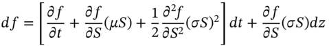
and ![]() , the dynamics of the derivative's price is (see Chapter 47):
, the dynamics of the derivative's price is (see Chapter 47):
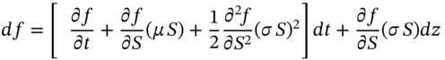
The SDE for the stock price and the derivatives price both depend on the same source of uncertainty, ![]() . Over a small interval of time, portfolio-A consisting of
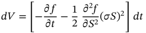
. Over a small interval of time, portfolio-A consisting of ![]() -stocks and holdings of bonds, can be made to replicate the payoff from the derivative security. The resulting equation (see Appendix 48) for the change in price of the derivative security does not depend on
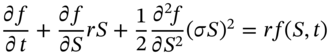
-stocks and holdings of bonds, can be made to replicate the payoff from the derivative security. The resulting equation (see Appendix 48) for the change in price of the derivative security does not depend on ![]() and is deterministic. This equation is known as the Black–Scholes PDE:
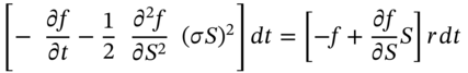
and is deterministic. This equation is known as the Black–Scholes PDE:
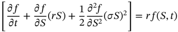
In Equation (48.4) the term in square brackets is similar to that in (48.3) but ![]() has been replaced by
has been replaced by ![]() . Therefore the solution to (48.4) for the option price does not depend on
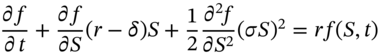
. Therefore the solution to (48.4) for the option price does not depend on ![]() – this is risk-neutral valuation (RNV), which is a consequence of no-arbitrage possibilities. When a stock pays dividends at a rate
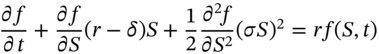
– this is risk-neutral valuation (RNV), which is a consequence of no-arbitrage possibilities. When a stock pays dividends at a rate ![]() the Black–Scholes PDE is:
the Black–Scholes PDE is:

The Black–Scholes PDE applies to any derivative security whose payoff depends on one underlying asset (and time). It therefore holds for plain vanilla European calls and puts, American options, and exotic options such as standard barrier options and lookback options. Sometimes the PDE (together with the boundary conditions for the option) results in a closed-form solution for the options price but if this is not possible, the PDE can be solved using finite difference methods.
Complex algebra is required to obtain the closed-form solution to (48.5) for the Black–Scholes call (or put) premium on a European option. Here we simply note that the solution to (48.5) requires specific boundary conditions. For example, for European calls and puts these are:
These boundary conditions when used with the PDE give the Black–Scholes closed-form solutions for European option prices:
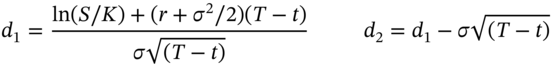
There are several solution methods available to solve the Black–Scholes PDE. In one method you take the Black–Scholes PDE (48.4) and transform it into a simpler PDE known (in physics) as the ‘heat equation’. (So called, because it explains the diffusion of heat through a metal bar with a heat source at one end.) The solution to the heat equation then gives the Black–Scholes formulas for European call and put premia.
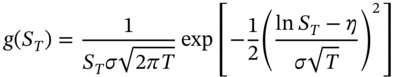
Another method to solve for the option price involves integration and we outline the steps below to obtain the Black–Scholes call premium. Assume ![]() where
where ![]() and the density function for
and the density function for ![]() is:
is:
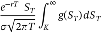
The call premium under risk-neutral pricing can written in terms of conditional expectations:
where![]() is an indicator function, that takes the value 1 if
is an indicator function, that takes the value 1 if ![]() and zero otherwise. The first and second terms in (48.9) can be written:
and zero otherwise. The first and second terms in (48.9) can be written:
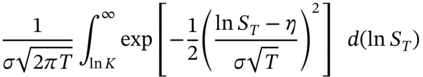
The integrals in (48.10) are not straightforward to evaluate but they result in the terms ![]() and
and ![]() which implies
which implies ![]() . The route to obtaining the Black–Scholes option pricing formula was a rather tortuous one (Finance Blog 48.1) – see Sudaram and Das (2015).
. The route to obtaining the Black–Scholes option pricing formula was a rather tortuous one (Finance Blog 48.1) – see Sudaram and Das (2015).
Although Black–Scholes was a major breakthrough, it is not always the case that a closed-form solution for the PDE is possible. What happens then? First, it is often possible to obtain a numerical solution to the Black–Scholes PDE (e.g. using finite difference methods). Alternatively we can use other numerical methods such as Monte Carlo simulation or the BOPM (under RNV) to price an option.
48.1.2 Does a Forward Contract Obey the Black–Scholes PDE?
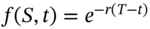
The price of any derivative security ![]() should satisfy the Black–Scholes PDE. We can illustrate this by considering a forward contract on a (non-dividend paying) stock. Using a no-arbitrage approach, we established that the value of a forward contract
should satisfy the Black–Scholes PDE. We can illustrate this by considering a forward contract on a (non-dividend paying) stock. Using a no-arbitrage approach, we established that the value of a forward contract ![]() at time
at time ![]() is:
is:
where ![]() = delivery price (= price
= delivery price (= price ![]() established at
established at ![]() ) and
) and ![]() = time to maturity. Does the above expression satisfy the Black–Scholes PDE? We have:
= time to maturity. Does the above expression satisfy the Black–Scholes PDE? We have:
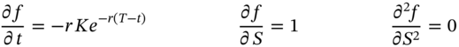
Substituting the above equations in the PDE (48.4):
And using (48.11) in (48.13) we see that forward price satisfies the Black–Scholes PDE.1
48.2 FINITE DIFFERENCE METHODS
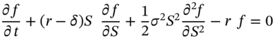
Finite difference methods provide an approximation to the continuous time PDE for the derivatives price, which can then be solved numerically. Consider the premium ![]() on a European put option on a (dividend paying) stock. The Black–Scholes PDE is:
on a European put option on a (dividend paying) stock. The Black–Scholes PDE is:
The explicit finite difference method approximates the above PDE and gives a set of equations that can be solved numerically for the option premium ![]() . To solve (48.14) we require some initial known values on the edges of the grid and these are given by the boundary conditions for the value of the put (e.g. the payoff at maturity, or when the stock price is zero). To illustrate the method consider the grid in Figure 48.1 which has time differences of
. To solve (48.14) we require some initial known values on the edges of the grid and these are given by the boundary conditions for the value of the put (e.g. the payoff at maturity, or when the stock price is zero). To illustrate the method consider the grid in Figure 48.1 which has time differences of ![]() along the horizontal axis and stock price changes of
along the horizontal axis and stock price changes of ![]() on the vertical axis.
on the vertical axis.
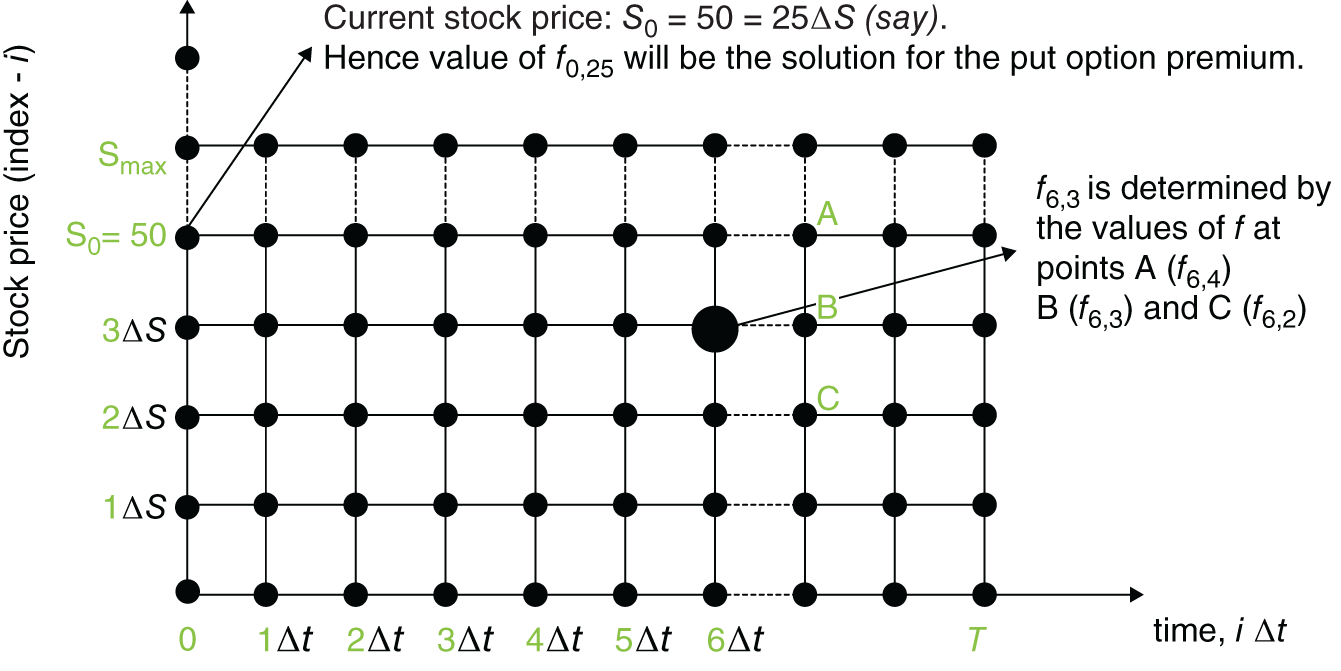
FIGURE 48.1 Finite difference
Each node on the grid will come to represent the option premium ![]() where the index-
where the index-![]() represents a particular time (x-axis) and the index-j represents the value of
represents a particular time (x-axis) and the index-j represents the value of ![]() (y-axis), hence:
(y-axis), hence:
The life of the option is ![]() years. The time axis is divided into
years. The time axis is divided into ![]() equally spaced intervals of length
equally spaced intervals of length ![]() , so there are
, so there are ![]() time periods:
time periods:
We now set the maximum value for S on the grid so that the put (with a strike of K) will have virtually zero value (this is an upper boundary for S) – for example, if ![]() then an upper boundary might be
then an upper boundary might be ![]() . Now consider
. Now consider ![]() equally spaced time intervals for S so that
equally spaced time intervals for S so that ![]() so the M + 1 stock prices in the grid are:
so the M + 1 stock prices in the grid are:
One of the nodes on the (left) vertical axis of Figure 48.1 will coincide with the current stock price ![]() (say) and the solved value for
(say) and the solved value for ![]() at this same node will be the option premium using the finite difference method. Now we are in a position to provide an approximation to the (differential) terms in the PDE (48.14). In the middle of the lattice the derivative
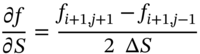
at this same node will be the option premium using the finite difference method. Now we are in a position to provide an approximation to the (differential) terms in the PDE (48.14). In the middle of the lattice the derivative ![]() can be approximated in three different ways (see Figure 48.2).
can be approximated in three different ways (see Figure 48.2).
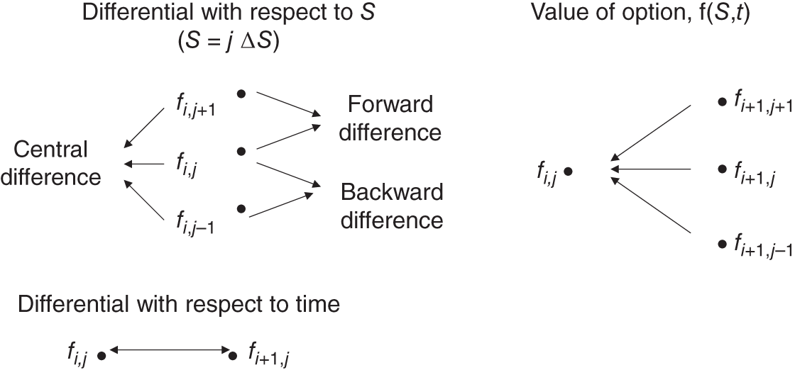
FIGURE 48.2 Use of grid points
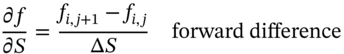
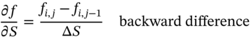
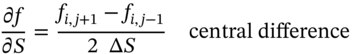
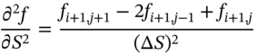
The other derivatives are (Figure 48.3):
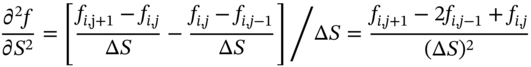
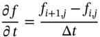
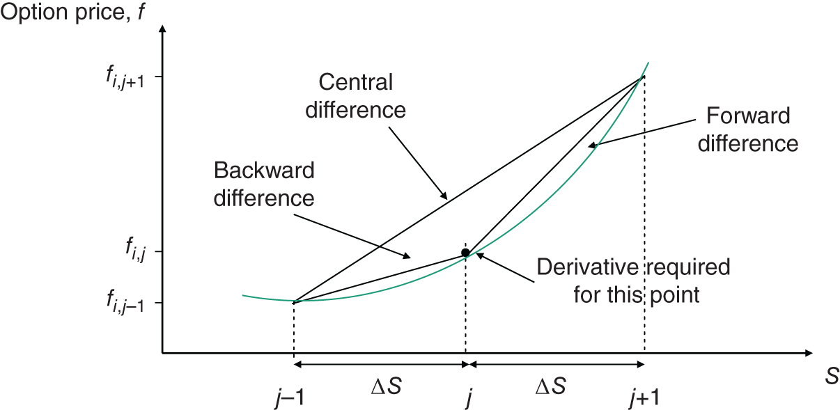
FIGURE 48.3 Approximations for ∂f/∂S
It is only the derivative ![]() that involves time. The explicit finite difference method simplifies the solution method by assuming that
that involves time. The explicit finite difference method simplifies the solution method by assuming that ![]() and
and ![]() at the point
at the point ![]() on the grid are the same as at point
on the grid are the same as at point ![]() so the central difference equation [16c] and equation [17a] become:
so the central difference equation [16c] and equation [17a] become:
Substituting (48.17b), (48.18a), and (48.18b) in the Black–Scholes PDE (48.14) and rearranging:
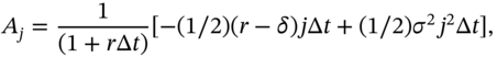
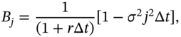
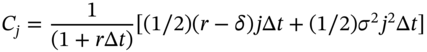
From (48.19) we can calculate the value of ![]() once we know the values of
once we know the values of ![]() for the three nodes at time (i + 1) – Figure 48.2. Hence once we have the terminal conditions for the option, we solve for
for the three nodes at time (i + 1) – Figure 48.2. Hence once we have the terminal conditions for the option, we solve for ![]() by working backwards through the grid (i.e. similar to solving the BOPM recursively). This is known as the explicit finite difference method. We know the value of the put for all nodes along the right boundary is
by working backwards through the grid (i.e. similar to solving the BOPM recursively). This is known as the explicit finite difference method. We know the value of the put for all nodes along the right boundary is ![]() , the value along the bottom boundary
, the value along the bottom boundary ![]() is K and along the top boundary (i.e.
is K and along the top boundary (i.e. ![]() ) the value of the put is zero.
) the value of the put is zero.
- Value of put at time T
(48.21a)

- Value of put when
 (48.21b)
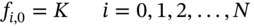
- Value of put when
 (48.21c)
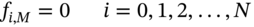
Equation (48.19) can then be used to determine the option premium ![]() at all points along the left hand edge of the grid, by working backwards from T. The value of
at all points along the left hand edge of the grid, by working backwards from T. The value of ![]() which corresponds to the same node as the current stock price is the solution for the option premium.
which corresponds to the same node as the current stock price is the solution for the option premium.
The main problem with the explicit finite difference method is that it may not converge. There are a wide variety of other numerical methods available (e.g. implicit finite difference method, Crank-Nicholson, Hopscotch etc.) which can overcome such problems (see Hull 2018).
Pricing an American put option is easily incorporated into the explicit finite difference method. Each time we calculate the grid value ![]() we check to see if
we check to see if ![]() . If
. If ![]() , then we replace
, then we replace ![]() at that node with
at that node with ![]() . We then repeat this procedure for all the nodes.
. We then repeat this procedure for all the nodes.
We could also use finite difference methods based on an approximation to the differential equation for ![]() (rather than for
(rather than for ![]() ) and this turns out to be slightly easier computationally. Although finite difference methods can be used for valuing American and European options they are more difficult to use when handling path-dependent options (e.g. where the payoff from the option depends on the past history of the underlying asset price). We then have to move to a ‘higher order’ problem since we have another state variable (e.g. the average value of the underlying for an Asian option). We therefore have to index the option value
) and this turns out to be slightly easier computationally. Although finite difference methods can be used for valuing American and European options they are more difficult to use when handling path-dependent options (e.g. where the payoff from the option depends on the past history of the underlying asset price). We then have to move to a ‘higher order’ problem since we have another state variable (e.g. the average value of the underlying for an Asian option). We therefore have to index the option value ![]() where k = new state variable. It is also the case that some finite difference methods are unstable and sensitive to rounding errors in the computational procedure. Because of these difficulties it is worth noting that analytic approximations for some options' prices are often available (e.g. for American options, Asian average price options).
where k = new state variable. It is also the case that some finite difference methods are unstable and sensitive to rounding errors in the computational procedure. Because of these difficulties it is worth noting that analytic approximations for some options' prices are often available (e.g. for American options, Asian average price options).
48.3 SUMMARY
- The stochastic process for the underlying stock
 and for the option premium
  have a common stochastic term
  , which can be eliminated by using delta hedging. This results in the deterministic Black–Scholes PDE for the option premium. The PDE depends on the risk-free rate but is independent of the actual growth rate of the stock price,
  – this is risk-neutral valuation.
 - In some cases the Black–Scholes PDE can be solved to give a closed-form solution for the option premium (e.g. for several types of European calls and puts).
- The Black–Scholes PDE can often be solved using numerical methods (e.g. finite difference methods). The procedure is similar to that used in the BOPM in that the PDE is initially ‘anchored’ by the boundary conditions implicit in the option contract and then the PDE is solved recursively.
- Generally speaking, numerical techniques to solve the Black–Scholes PDE for many European options is usually accurate and speedy, even if the model involves more than three variables or ‘dimensions’ (e.g. time and two underlying stochastic variables S1 and S2). When the dimension of the problem is greater than three, then MCS tends to be a more efficient method of pricing a European option.
APPENDIX 48: DERIVATION OF BLACK–SCHOLES PDE
We derive the Black–Scholes PDE for the derivative security ![]() (on a stock which pays no dividends), using two alternative replication portfolios, over short intervals of time. The analysis closely follows that used in earlier chapters to price options using the BOPM. Here we simply repeat that analysis in a continuous time framework.
(on a stock which pays no dividends), using two alternative replication portfolios, over short intervals of time. The analysis closely follows that used in earlier chapters to price options using the BOPM. Here we simply repeat that analysis in a continuous time framework.
Case A: Replication using stocks and (zero coupon) bonds
We replicate the price dynamics of the derivative security (e.g. call or put) using stocks and zero-coupon bonds (risk-free asset). Assume the stock price follows a GBM and the bond price is deterministic:
From Ito's lemma, the price of the derivative security ![]() follows the SDE:
follows the SDE:
In our replication portfolio we hold ![]() stocks and
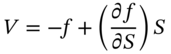
stocks and ![]() bonds. The value of the replication portfolio
bonds. The value of the replication portfolio ![]() is set equal to the value of the derivative security (at any time t):
is set equal to the value of the derivative security (at any time t):
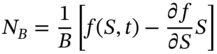
Hence the number of bonds held is:
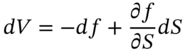
The instantaneous change in the value of the replication portfolio is:
Substituting from (48.A.1) and (48.A.2) in (48.A.6) gives:
We require the change in value of the replication portfolio to equal the change in value of the derivative itself:
Equating the coefficients on ![]() in Equation (48.A.7) and (48.A.3) implies:
in Equation (48.A.7) and (48.A.3) implies:
Thus the number of stocks to hold at time t equals the option's delta, ![]() . From Equations (48.A.5) and (48.A.9):
. From Equations (48.A.5) and (48.A.9):
It remains to equate the coefficients on ![]() . Substituting for
. Substituting for ![]() in (48.A.7), using
in (48.A.7), using ![]() and then equating with (48.A.3) for terms in
and then equating with (48.A.3) for terms in ![]() gives:
gives:
Rearranging (48.A.11) we have the Black–Scholes PDE for the derivative security ![]() (on a stock which pays no dividends):
(on a stock which pays no dividends):
The PDE equation (48.A.12a) is deterministic and independent of ![]() the growth rate of the stock price, so the option price does not depend on
the growth rate of the stock price, so the option price does not depend on ![]() . For a stock which pays dividends, the growth of the stock price (in a risk-neutral world) is not equal to
. For a stock which pays dividends, the growth of the stock price (in a risk-neutral world) is not equal to ![]() but to
but to ![]() , where
, where ![]() is the growth rate of dividends, hence the PDE becomes:
is the growth rate of dividends, hence the PDE becomes:
Case B: Risk-free Portfolio-B (Stock Pays No Dividends)
The Black–Scholes PDE can be derived in a simpler fashion if we assume we already know how to construct a risk-free portfolio. Assume the risk-free Portfolio-B consists of a long position in ![]() stocks (where
stocks (where ![]() ) and a short position in the derivative security (
) and a short position in the derivative security (![]() ) with current price
) with current price ![]() . The value of portfolio-B is:
. The value of portfolio-B is:
Substitute in (48.A.14) for ![]() from Equation (48.A.1) and for
from Equation (48.A.1) and for ![]() from Ito's equation (48.A.3). Crucially, the term in
from Ito's equation (48.A.3). Crucially, the term in ![]() cancels out and we are left with:
cancels out and we are left with:
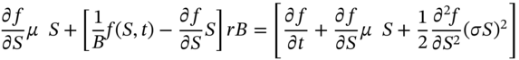
The change in value of portfolio-B is deterministic so risk-free arbitrage profits are possible unless portfolio-B earns the risk-free rate:
Substituting from Equation (48.A.15) and (48.A.13) in (48.A.16):
A simple rearrangement of (48.A.17) gives the Black–Scholes PDE, Equation (48.A.12).
Dividend Paying Stock
If we hold ![]() stocks which pay a continuous dividend at the (proportionate) rate
stocks which pay a continuous dividend at the (proportionate) rate ![]() , then the (dollar) dividend paid out over time interval
, then the (dollar) dividend paid out over time interval ![]() is
is ![]() , which needs to be added to the right hand side of (48.A.15). The rest of the analysis is unchanged and the Black–Scholes PDE for an option on a dividend paying stock is:
, which needs to be added to the right hand side of (48.A.15). The rest of the analysis is unchanged and the Black–Scholes PDE for an option on a dividend paying stock is:
EXERCISES
Question 1
Use Ito's lemma to shown that if ![]() follows a GBM with drift rate
follows a GBM with drift rate ![]() and variance,
and variance, ![]() then the futures price
then the futures price ![]() follows a GBM with drift rate
follows a GBM with drift rate ![]() (where
(where ![]() is the risk-free rate) and variance,
is the risk-free rate) and variance, ![]() .
.
Question 2
If the change in the stock price follows a GBM, ![]() , use Ito's lemma to show that
, use Ito's lemma to show that ![]() follows
follows ![]() .
.
Question 3
What assumptions are made in moving from an SDE for the option price to the Black–Scholes PDE?
Question 4
What is a partial differential equation (PDE)? What is the key difference between a SDE and a PDE?
Question 5
What are the key strengths and weaknesses in calculating European option premia using finite difference methods? What role is played by boundary conditions?
NOTE
- 1 Also note that it is trivial to show that a zero coupon bond (with face value of $1) and
 satisfies the Black–Scholes PDE. This is left as a simple exercise for the reader.