CHAPTER 21
BOPM: Introduction
Aims
- To demonstrate how the binomial option pricing model (BOPM), is used to determine option premia by establishing a risk-free arbitrage portfolio consisting of a position in stocks and the option – this is delta hedging.
- To show how delta hedging and the no-arbitrage approach can be interpreted in terms of risk-neutral valuation (RNV), which allows us to price options using a simple backward recursion.
- To demonstrate how RNV leads to other useful approaches to pricing options such as Monte Carlo simulation.
We present a detailed account of the BOPM for pricing options using the no-arbitrage principle – the option is priced so that traders faced with this ‘BOPM price’ cannot undertake trades which result in risk-free profits. We construct a risk-free portfolio from two risky assets, namely calls and stocks. Using the principle of delta hedging, whereby the proportions held in stocks and the option gives a risk-free portfolio (over small intervals of time) – we obtain the BOPM formula for the price of the option. We then interpret the BOPM formula in terms of risk-neutral valuation (RNV). Using insights from RNV we can then price an option without going through all the details involved in delta hedging and forming a ‘risk-free arbitrage portfolio’ – instead we price the option directly by using the BOPM formula and ‘backward recursion’.
21.1 ONE-PERIOD BOPM
To understand delta hedging and risk-neutral valuation we first price a European call option (on a non-dividend paying stock), which has one period to expiration. The basic idea is to construct a portfolio consisting of the call option and some stocks, so that the portfolio is risk-free (over a small interval of time).
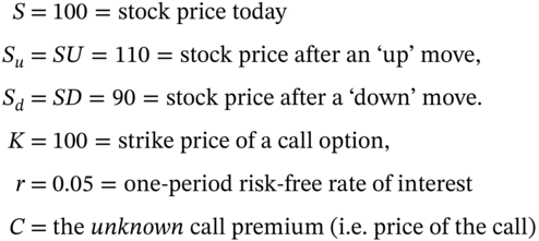
The current stock price is ![]() and the stock pays no dividends. Consider a one-period problem where there are only two possible outcomes for the stock price at
and the stock pays no dividends. Consider a one-period problem where there are only two possible outcomes for the stock price at ![]() , namely an ‘up’ move with
, namely an ‘up’ move with ![]() and a ‘down’ move with
and a ‘down’ move with ![]() , hence:
, hence:
Suppose the ‘real world’ probability of the stock price moving up or down is ![]() , so the ‘real world’ expected stock price at
, so the ‘real world’ expected stock price at ![]() is
is ![]() and since
and since ![]() the expected stock return
the expected stock return![]() . As we see below, somewhat surprisingly, neither the ‘real world’ probability
. As we see below, somewhat surprisingly, neither the ‘real world’ probability ![]() of a rise in the stock price nor the ‘real world’ expected return on the stock
of a rise in the stock price nor the ‘real world’ expected return on the stock ![]() determine the call premium.
determine the call premium.
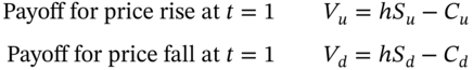
The payoffs when holding either one stock or one long call are given in Figure 21.1. Note that if the payoff to a long call is +10 (at ![]() ), then the payoff to a short (sold/written) call is –10. The difference between the two possible outcomes for the stock is
), then the payoff to a short (sold/written) call is –10. The difference between the two possible outcomes for the stock is ![]() and for the call is
and for the call is ![]() . We define the hedge ratio as
. We define the hedge ratio as ![]() .
.
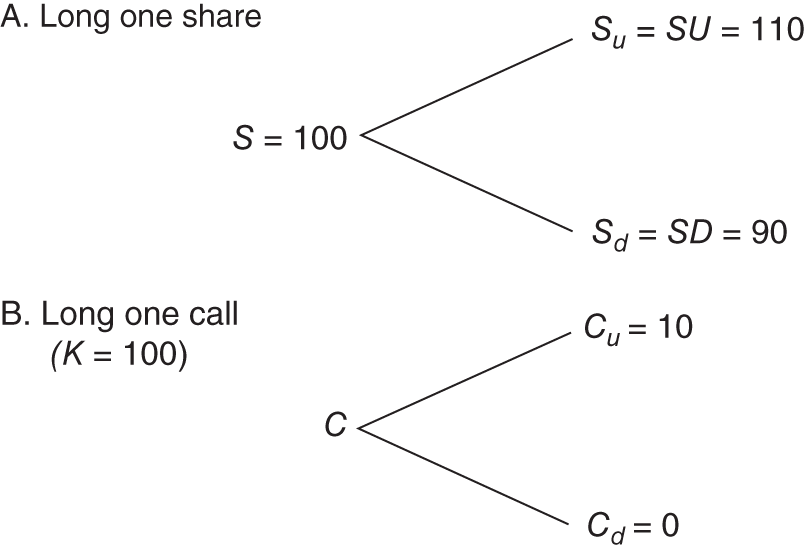
FIGURE 21.1 One-period BOPM – call
Below, we see that if today ![]() Ms Arb sells one call and buys
Ms Arb sells one call and buys ![]() stock (or alternatively if Ms Arb sells 100 calls and buys 50 stocks) then she has set up a risk-free portfolio (over a small interval of time). To be ‘risk-free’ this portfolio must have a known value at
stock (or alternatively if Ms Arb sells 100 calls and buys 50 stocks) then she has set up a risk-free portfolio (over a small interval of time). To be ‘risk-free’ this portfolio must have a known value at ![]() no matter what the values of the stock price and call premium are at
no matter what the values of the stock price and call premium are at ![]() . To set up this ‘hedge portfolio’ involves a cash outlay at time
. To set up this ‘hedge portfolio’ involves a cash outlay at time ![]() but because the payoff at
but because the payoff at ![]() is known, Ms Arb's hedge portfolio must have a return equal to the risk-free rate – or profitable arbitrage opportunities are possible. Consider the payoff to portfolio-A where Ms Arb is long 1/2-stock and short 1-call.
is known, Ms Arb's hedge portfolio must have a return equal to the risk-free rate – or profitable arbitrage opportunities are possible. Consider the payoff to portfolio-A where Ms Arb is long 1/2-stock and short 1-call.
Payoff to Portfolio-A: long 1/2 stock, short 1-call
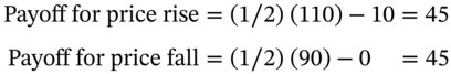
The payoff to portfolio-A at ![]() is known with certainty, no matter what the outcome for the stock price (i.e. either 110 or 90). Ms Arb has created a risk-free portfolio using a hedge ratio of
is known with certainty, no matter what the outcome for the stock price (i.e. either 110 or 90). Ms Arb has created a risk-free portfolio using a hedge ratio of ![]() . The cost of constructing portfolio-A at
. The cost of constructing portfolio-A at ![]() is the cost of buying the stocks less the receipt from the sale of the call, that is,
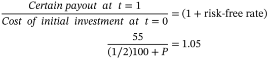
is the cost of buying the stocks less the receipt from the sale of the call, that is, ![]() . Portfolio-A is risk-free and if there are to be no arbitrage profits to be made, portfolio-A must earn the risk-free rate:
. Portfolio-A is risk-free and if there are to be no arbitrage profits to be made, portfolio-A must earn the risk-free rate:
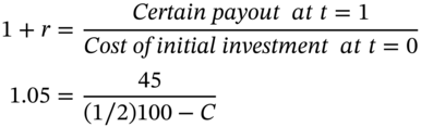
Therefore the ‘fair’, ‘correct’ or ‘no-arbitrage’ price of the call is ![]() . Alternatively, if you borrow
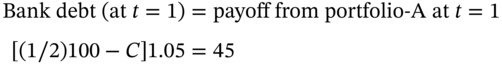
. Alternatively, if you borrow ![]() to set up portfolio-A then you will owe the bank
to set up portfolio-A then you will owe the bank ![]() at
at ![]() and for no arbitrage profits to be made, this must equal the (known) payoff of 45 at
and for no arbitrage profits to be made, this must equal the (known) payoff of 45 at ![]() :
:
Again the solution to Equation (21.2) is ![]()
21.1.1 Arbitrage: Overpriced Call
The fair price of the option is ![]() – otherwise risk-free arbitrage profits can be made. To see this, suppose the actual quoted option premium (by all option traders) is
– otherwise risk-free arbitrage profits can be made. To see this, suppose the actual quoted option premium (by all option traders) is ![]() which exceeds the BOPM ‘fair price’
which exceeds the BOPM ‘fair price’ ![]() – the call is overpriced. Ms Arb spots this pricing anomaly. As usual, Ms Arb ‘sells high and buys low’. At
– the call is overpriced. Ms Arb spots this pricing anomaly. As usual, Ms Arb ‘sells high and buys low’. At ![]() , she sells (writes) the overpriced call and receives
, she sells (writes) the overpriced call and receives ![]() and hedges by purchasing
and hedges by purchasing ![]() a stock at
a stock at ![]() , at a net cost of $40, which she borrows from the bank. The guaranteed cash value of this hedged ‘portfolio-A’ at
, at a net cost of $40, which she borrows from the bank. The guaranteed cash value of this hedged ‘portfolio-A’ at ![]() is $45 (no matter whether the stock price goes up or down) and as she owes the bank
is $45 (no matter whether the stock price goes up or down) and as she owes the bank ![]() she makes an arbitrage profit of $3.
she makes an arbitrage profit of $3.
Viewed slightly differently, the net cost of setting up portfolio-A at ![]() is
is ![]() and if Ms Arb uses her ‘own funds’ of $40 today then her return is
and if Ms Arb uses her ‘own funds’ of $40 today then her return is ![]() , which is in excess of the risk-free (borrowing) rate of 5% – again indicating risk-free arbitrage profits.
, which is in excess of the risk-free (borrowing) rate of 5% – again indicating risk-free arbitrage profits.
Note that there will be lots of traders who try to implement this risk-free, yet profitable strategy. Selling calls would tend to lead to a fall in the quoted price of ![]() and move it towards the ‘fair’ no-arbitrage price
and move it towards the ‘fair’ no-arbitrage price ![]() . Hence, we expect the quoted call premium to deviate from its (BOPM) fair price only by a small amount and for any discrepancies to be quickly eliminated by the actions of arbitrageurs.
. Hence, we expect the quoted call premium to deviate from its (BOPM) fair price only by a small amount and for any discrepancies to be quickly eliminated by the actions of arbitrageurs.
21.1.2 Arbitrage: Underpriced Call
Consider how to make arbitrage profits if the call is temporarily underpriced at a quoted price ![]() . Ms Arb buys low, sells high. So today, she buys the call at
. Ms Arb buys low, sells high. So today, she buys the call at![]() and hedges this position by short-selling
and hedges this position by short-selling ![]() stock, for which she receives
stock, for which she receives ![]() at
at ![]() . Her net cash inflow at
. Her net cash inflow at ![]() is
is ![]() . This can be invested at the risk-free rate to give receipts at
. This can be invested at the risk-free rate to give receipts at ![]() of
of ![]() . Ms Arb's hedged portfolio will be worth minus $45 at
. Ms Arb's hedged portfolio will be worth minus $45 at ![]() – that is, when she closes out all her short stock and long call positions she will have lost $45 (regardless of whether the stock price rises or falls). Hence she makes an overall profit at
– that is, when she closes out all her short stock and long call positions she will have lost $45 (regardless of whether the stock price rises or falls). Hence she makes an overall profit at ![]() of
of ![]() .
.
21.1.2.1 Formal Derivation
We now derive the price of the call option algebraically. The two outcomes for the stock price are ![]() and
and ![]() (where in our example
(where in our example ![]() and
and ![]() as shown in Figure 21.1).1 Let:
as shown in Figure 21.1).1 Let:
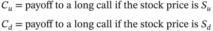
Hence:
Portfolio-A: long
![]() -stocks, short 1-call
-stocks, short 1-call
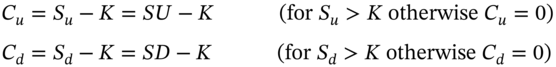
The payoff to a long call at ![]() is
is ![]() or
or ![]() so the payoff to a short call is
so the payoff to a short call is ![]() or
or ![]() . For the two payoffs to be equal:
. For the two payoffs to be equal:
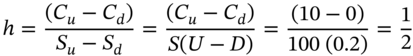
In the above analysis we are short one call and (21.4) indicates that the hedge will then involve going long![]() -stocks. The formula for the hedge ratio
-stocks. The formula for the hedge ratio ![]() in (21.4) is the change in value of the option divided by the change in value of the stock and this is the option's ‘delta’ – hence this approach is called delta hedging. Given the risk-free portfolio-A, we determine the call premium
in (21.4) is the change in value of the option divided by the change in value of the stock and this is the option's ‘delta’ – hence this approach is called delta hedging. Given the risk-free portfolio-A, we determine the call premium ![]() by equating the amount of bank debt owed at
by equating the amount of bank debt owed at ![]() (due to the cost of setting up portfolio-A at
(due to the cost of setting up portfolio-A at ![]() ), with the known payoff from portfolio-A at
), with the known payoff from portfolio-A at ![]() :
:
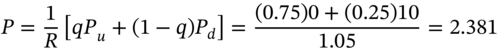
Substituting from Equation (21.4) for ![]() and (carefully) rearranging, the BOPM equation for the call premium is:
and (carefully) rearranging, the BOPM equation for the call premium is:
and
21.2 RISK-NEUTRAL VALUATION
Note that the formula for the call premium does not depend on the ‘real world’ probability ![]() of an ‘up’ move for the stock price (and hence is independent of the ‘real world’ expected return
of an ‘up’ move for the stock price (and hence is independent of the ‘real world’ expected return ![]() on the stock). In the formula for the call premium the ‘weights’ applied to the two option payoffs
on the stock). In the formula for the call premium the ‘weights’ applied to the two option payoffs ![]() and
and ![]() are
are ![]() and
and ![]() (which sum to unity), but there is little intuitive insight at present to be gleaned from Equation (21.6c) for
(which sum to unity), but there is little intuitive insight at present to be gleaned from Equation (21.6c) for ![]() .
.
The ‘weight’ ![]() is known as the risk-neutral probability of a rise in the stock price, which must not be confused with the actual ‘real world’ probability of a rise in the stock price
is known as the risk-neutral probability of a rise in the stock price, which must not be confused with the actual ‘real world’ probability of a rise in the stock price ![]() . The risk-neutral probability is simply a number which lies between 0 and 1 and is derived under the assumption that portfolio-A is risk-free.2 The expected payoff to the option, using risk-neutral probabilities is:
. The risk-neutral probability is simply a number which lies between 0 and 1 and is derived under the assumption that portfolio-A is risk-free.2 The expected payoff to the option, using risk-neutral probabilities is:
In some ways the term ‘risk-neutral probability’ could be misleading since it appears to imply that we are assuming investors are ‘risk neutral’ and hence do not care about risk. Investors in options do care about the level of risk they hold but in the BOPM they can set up a risk-free hedge portfolio and by definition this has zero risk. An alternative is to call ![]() , an equivalent martingale probability and the latter is used frequently in the continuous time literature. However, we will stick with the more commonly used term, ‘risk-neutral probability’. Using Equation (21.6a) we can price the option using the risk-neutral probability
, an equivalent martingale probability and the latter is used frequently in the continuous time literature. However, we will stick with the more commonly used term, ‘risk-neutral probability’. Using Equation (21.6a) we can price the option using the risk-neutral probability ![]() and this method of pricing is known as risk-neutral valuation (RNV) and it plays a major role in the pricing of all types of options. Hence we can now state:
and this method of pricing is known as risk-neutral valuation (RNV) and it plays a major role in the pricing of all types of options. Hence we can now state:
The call premium
is the expected payoff at maturity, where the expectation uses risk-neutral probabilities (
,
) and the expected payoff is discounted using the risk-free rate.
![]() is not a ‘real probability’ it is a ‘pseudo-probability’:
is not a ‘real probability’ it is a ‘pseudo-probability’: ![]() lies between 0 and 1 and the sum of
lies between 0 and 1 and the sum of ![]() and
and ![]() for the two possible outcomes is 1. But why is
for the two possible outcomes is 1. But why is ![]() known as a risk-neutral probability? We use a ‘what if’ argument here, to help explain the term, ‘risk-neutral probability’. If the probability of an ‘up’ move equals
known as a risk-neutral probability? We use a ‘what if’ argument here, to help explain the term, ‘risk-neutral probability’. If the probability of an ‘up’ move equals ![]() , then what would we expect the stock price to be at
, then what would we expect the stock price to be at ![]() ? This is given by:
? This is given by:
where ![]() is the expected value, using risk-neutral probabilities.
is the expected value, using risk-neutral probabilities.
But the initial stock price is ![]() , so if we interpret
, so if we interpret![]() as the probability of an ‘up’ move then this implies that the stock price (in the BOPM) is expected to grow at
as the probability of an ‘up’ move then this implies that the stock price (in the BOPM) is expected to grow at ![]() . But this is also the value of the risk-free rate,
. But this is also the value of the risk-free rate, ![]() . Hence, the no-arbitrage BOPM price for the option given by Equation (21.6a) is consistent with the assumption that the stock price grows at a rate (or has an expected return) equal to the risk-free interest rate. Confused? Yes, RNV is a tricky concept. However, it turns out to be a brilliant insight since it allows us to price very complex options by:
. Hence, the no-arbitrage BOPM price for the option given by Equation (21.6a) is consistent with the assumption that the stock price grows at a rate (or has an expected return) equal to the risk-free interest rate. Confused? Yes, RNV is a tricky concept. However, it turns out to be a brilliant insight since it allows us to price very complex options by:
- using the ‘pseudo-probabilities’
 , to ‘weight’ the option payoffs, to give an ‘expected payoff’ to the option (in a risk-neutral world).
 - Discount these expected payoffs using the risk-free rate, to give the correct no-arbitrage price of the option.
Rather miraculously we obtain the correct no-arbitrage ‘real world’ option price using the above two assumptions, even though in the real world the stock price does not grow at the risk-free rate.3 As long as we use our two ‘tricks’, they compensate for each other and enable us to obtain the ‘fair’ or ‘correct’ (i.e. no-arbitrage) option price, in the real world. What do we mean by ‘correct’? We mean a price for the option that does not allow any risk-free arbitrage profits to be made in the ‘real world’ – now that does sound sensible and ‘real’.
Finally note that in Equation (21.6a) neither the actual probability ![]() of a rise in the stock price nor the real world growth rate of the stock
of a rise in the stock price nor the real world growth rate of the stock ![]() , nor the risk preferences of investors, enter into the calculation of the price of the call. Hence all investors, regardless of their differing degrees of risk aversion or their different guesses about the ‘real world’ probability of a rise or fall in future stock prices can agree on the ‘fair’ or ‘correct’ price for a call option.
, nor the risk preferences of investors, enter into the calculation of the price of the call. Hence all investors, regardless of their differing degrees of risk aversion or their different guesses about the ‘real world’ probability of a rise or fall in future stock prices can agree on the ‘fair’ or ‘correct’ price for a call option.
21.2.1 RNV and No-arbitrage
We can use some more tricks. If ![]() really is a risk-neutral probability, then in a risk-neutral world, the expected return on a stock must equal the risk free rate and hence
really is a risk-neutral probability, then in a risk-neutral world, the expected return on a stock must equal the risk free rate and hence ![]() must satisfy:
must satisfy:
From Equation (21.8) we can immediately deduce that ![]() which we know to be true from our ‘no-arbitrage’ approach. Similarly, in a risk-neutral world the call option has a
which we know to be true from our ‘no-arbitrage’ approach. Similarly, in a risk-neutral world the call option has a ![]() chance of being worth
chance of being worth ![]() and a 0.25 chance of being worth
and a 0.25 chance of being worth ![]() . Hence its expected value (at
. Hence its expected value (at ![]() ) in this risk-neutral world is:
) in this risk-neutral world is:
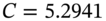
Discounting at the risk-free rate, the call premium at ![]() in a risk-neutral world is:
in a risk-neutral world is:
Thus, using RNV the BOPM Equation (21.6a) gives the same value for C as when we use the full ‘no-arbitrage’ approach. This establishes the equivalence of the two approaches. When pricing an option, if you interpret ![]() as the probability of an ‘up’ move, this is equivalent to assuming the expected stock return is equal to the risk-free rate
as the probability of an ‘up’ move, this is equivalent to assuming the expected stock return is equal to the risk-free rate ![]() – that is, you are in a risk-neutral world. However, the resulting value for the option premium using Equation (21.6a) is valid in the real world, since Equation (21.6a) is consistent with no risk-free arbitrage profits. This is the principle of RNV.
– that is, you are in a risk-neutral world. However, the resulting value for the option premium using Equation (21.6a) is valid in the real world, since Equation (21.6a) is consistent with no risk-free arbitrage profits. This is the principle of RNV.
Using RNV we could say that the call premium at any time ![]() is given by:
is given by:
where![]() is the expected payoff to the option at time
is the expected payoff to the option at time ![]() , and the expectation
, and the expectation ![]() assumes we are in a risk-neutral world – that is, the stock price grows at the risk-free rate. This is also the basis for pricing options using Monte-Carlo simulation (MCS), as we see later. MCS involves simulating the stock price assuming the expected stock return equals the risk-free rate (
assumes we are in a risk-neutral world – that is, the stock price grows at the risk-free rate. This is also the basis for pricing options using Monte-Carlo simulation (MCS), as we see later. MCS involves simulating the stock price assuming the expected stock return equals the risk-free rate (![]() ), calculating the expected payoff from the option at maturity
), calculating the expected payoff from the option at maturity ![]() and discounting this expected payoff using the risk-free rate.
and discounting this expected payoff using the risk-free rate.
21.3 DETERMINANTS OF CALL PREMIUM
21.3.1 Call Premium and Stock Returns
Somewhat counter-intuitively the binomial pricing formula implies that if we have two otherwise identical call options (i.e. same strike price, expiration date, and same stock return volatility) but the underlying stock-A for one of the options has a ‘real world’ expected return of ![]() = 0, while the other stock-B, has an expected return of
= 0, while the other stock-B, has an expected return of ![]() p.a. (say), then the two options will have exactly the same call price. This is because in each case we can create a risk-free hedge portfolio, which by arbitrage arguments can only earn the risk-free rate. Put another way, the call premium is independent of the ‘real world’ expected return of the underlying stock,
p.a. (say), then the two options will have exactly the same call price. This is because in each case we can create a risk-free hedge portfolio, which by arbitrage arguments can only earn the risk-free rate. Put another way, the call premium is independent of the ‘real world’ expected return of the underlying stock, ![]() .
.
21.3.2 Call Premium and Volatility
Note, however, that we are not saying that the call premium is independent of the volatility of the underlying stock (represented in the BOPM by ![]() or equivalently ‘
or equivalently ‘![]() ’, which enters the definition of
’, which enters the definition of ![]() ).4 Expected growth and volatility are very different concepts. After all, we can have a stock price with an expected growth (return) of zero but we may feel that the range of possible outcomes (around its expected value of zero) is very large. In our simple one-period model the call premium does depend on the range of possible values for
).4 Expected growth and volatility are very different concepts. After all, we can have a stock price with an expected growth (return) of zero but we may feel that the range of possible outcomes (around its expected value of zero) is very large. In our simple one-period model the call premium does depend on the range of possible values for ![]() – that is on
– that is on ![]() and
and ![]() – which measure the volatility of the stock price in the BOPM (and as we have seen, volatility also plays a key role in the Black–Scholes option price formulas).
– which measure the volatility of the stock price in the BOPM (and as we have seen, volatility also plays a key role in the Black–Scholes option price formulas).
To show that the call premium depends positively on the volatility of the stock, go back to our original example where ![]() and
and ![]() and the ‘volatility’
and the ‘volatility’ ![]() . Now change the volatility of the stock price, by assuming
. Now change the volatility of the stock price, by assuming ![]() and
and ![]() , so the volatility increases to
, so the volatility increases to ![]() . The ‘real world’ expected stock price (at
. The ‘real world’ expected stock price (at ![]() ) with
) with ![]() is
is ![]() and the ‘real world’ expected return remains unchanged at
and the ‘real world’ expected return remains unchanged at ![]() .
.
The payoff to the call is either ![]() or
or ![]() . Also
. Also ![]() and hence using Equation (21.6a) the call premium
and hence using Equation (21.6a) the call premium ![]() ,5 which is higher than the call premium of
,5 which is higher than the call premium of ![]() (when we assumed stock price volatility was lower (i.e.
(when we assumed stock price volatility was lower (i.e. ![]() )).
)).
Of course, the above examples have two key simplifying assumptions, namely that there are only two possible outcomes for the stock price and that the option expiration is after one period. However, by extending the number of branches in the binomial ‘tree’ we can obtain a large number of possible outcomes for the stock price. If we consider each ‘branch’ as representing a short time period, then conceptually we can see how the BOPM ‘approaches’ a continuous time formulation, which forms the basis of the famous Black–Scholes approach.
21.4 PRICING A EUROPEAN PUT OPTION
We can price a one-period put option by constructing a similar risk-free portfolio of stocks and the put. But this time the risk-free portfolio-B is obtained by going long some stocks and simultaneously going long one put. So, if S falls the loss on the stock will be offset by the gain on the put, making the portfolio of ‘stock+put’, risk-free. The payoff to the put is max (0, K – ST). If ![]() (as before, Figure 21.2) then for
(as before, Figure 21.2) then for ![]() the put payoff is
the put payoff is ![]() and for
and for ![]() we have
we have ![]() .
.
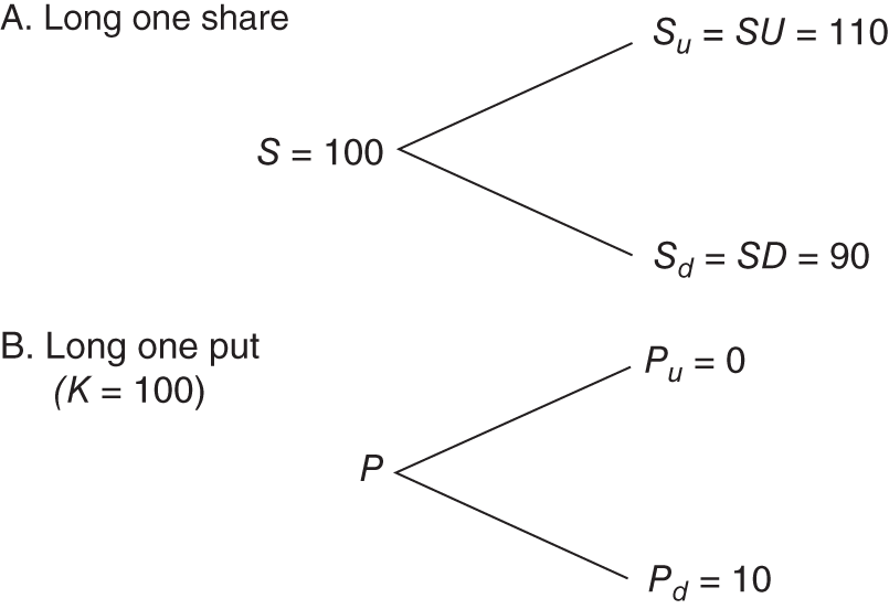
FIGURE 21.2 One-period BOPM – put
The hedge ratio is ![]() . For each long put option a delta hedge requires the purchase of ½ stock. The cost of setting up the delta hedge at
. For each long put option a delta hedge requires the purchase of ½ stock. The cost of setting up the delta hedge at ![]() is
is ![]() and the payoff at
and the payoff at ![]() is:
is:
Payoff to Portfolio-B: long 1/2-stock + long 1-put
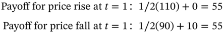
Equating the return on the risk-free hedge portfolio-B to the risk-free rate gives:
Hence ![]() . Alternatively using the BOPM risk-neutral valuation formula, we directly obtain the put premium:
. Alternatively using the BOPM risk-neutral valuation formula, we directly obtain the put premium:
where (again) ![]() . Equation (21.13) has the same form as that for the call premium except that we use the put payoffs
. Equation (21.13) has the same form as that for the call premium except that we use the put payoffs ![]() and
and ![]() . The BOPM put premium
. The BOPM put premium ![]() can be checked by using put–call parity.
can be checked by using put–call parity.
21.5 SUMMARY
- By constructing a risk-free portfolio consisting of the option and the underlying stock and delta hedging, the BOPM can be used to determine the ‘no-arbitrage’ call and put premia.
- The hedge ratio is given by the delta of the option.
- The call and put premia are determined by (i) the current stock price
 , (ii) the risk-free rate
  , (iii)
  and
and  (which can be shown to determine the stock return volatility), (iv)
 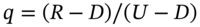 , the risk-neutral probability, and (v) the time to maturity,
  . The option premia do not depend on the real-world expected stock return,
  .
. - The parameter
 can be interpreted as a risk-neutral probability of an ‘up’ move and two key results follow. First, the option premium (C or P) given by the BOPM is the expected payoff to the option at
  , using risk-neutral probabilities
  and the payoff is discounted at the risk-free rate. Second, the BOPM formula Equation (21.6) derived via arbitrage is consistent with the assumption that the expected growth rate of the stock price equals the risk-free rate. This is risk-neutral valuation (RNV).
 - RNV provides a way of obtaining the correct value for option premia using the BOPM Equation (21.6), which involves backward recursion – this considerably simplifies the calculations. But behind this approach is the assumption that options traders have eliminated any risk-free arbitrage opportunities.
- RNV also leads to other useful approaches to pricing options such as Monte Carlo simulation.
APPENDIX 21: NO-ARBITRAGE CONDITIONS
We show that there are arbitrage opportunities if the inequalities ![]() do not hold for the underlying asset (stock), with current price S. First, note that it is always the case that
do not hold for the underlying asset (stock), with current price S. First, note that it is always the case that ![]() (by construction). Consider the arbitrage opportunity when
(by construction). Consider the arbitrage opportunity when ![]() (and hence
(and hence ![]() ). Here the outcome for either U or D is greater than the cost of borrowing. Hence at
). Here the outcome for either U or D is greater than the cost of borrowing. Hence at ![]() , borrow S (e.g. bank loan) and buy the stock for S – the net cash flow is zero (Table 21.A.1). The outcome for either U or D at
, borrow S (e.g. bank loan) and buy the stock for S – the net cash flow is zero (Table 21.A.1). The outcome for either U or D at ![]() is a debt to the bank of RS. But at
is a debt to the bank of RS. But at ![]() the value of the long position in the stock is either SU or SD and the net position is either
the value of the long position in the stock is either SU or SD and the net position is either ![]() or
or ![]() . This is an arbitrage opportunity as the net cash flow at
. This is an arbitrage opportunity as the net cash flow at ![]() is zero but there is a positive cash flow at
is zero but there is a positive cash flow at ![]() , for both the U and D outcomes.
, for both the U and D outcomes.
TABLE 21.A.1 Case A: U > D > R
| Action | Cash Flow, |
Cash Flow ‘Up-Move’, |
Cash Flow ‘Down Move’, |
| Borrow $S @ R | −S | −SR | −SR |
| Buy stock @ S | +S | SU | SD |
| Net cash flow | 0 |
|
|
For ![]() , the risk-free rate exceeds the return on the stock for both the U and D outcomes. The arbitrage strategy at
, the risk-free rate exceeds the return on the stock for both the U and D outcomes. The arbitrage strategy at ![]() involves short-selling the stock at S and investing the proceeds (in a bank deposit) which accrues to RS (Table 21.A.2). The cost of buying back the stock at
involves short-selling the stock at S and investing the proceeds (in a bank deposit) which accrues to RS (Table 21.A.2). The cost of buying back the stock at ![]() is either SU or SD. Hence there is a zero cash flow at
is either SU or SD. Hence there is a zero cash flow at ![]() and a positive cash flow of either
and a positive cash flow of either ![]() or
or ![]() at
at ![]() .
.
TABLE 21.A.2 Case B: D < U < R
| Action | Cash Flow, |
Cash Flow ‘Up-Move’, |
Cash Flow ‘Down Move’, |
| Short-sell stock @ S | +S | −SU | −SD |
| Invest $S @ R | −S | SR | SR |
| Net cash flow | 0 |
|
|
EXERCISES
Question 1
Show that the risk-neutral probability ![]() in the (one-period) BOPM is consistent with the assumption that the underlying stock price S (which pays no dividends) grows at the risk-free rate.
in the (one-period) BOPM is consistent with the assumption that the underlying stock price S (which pays no dividends) grows at the risk-free rate. ![]() , where
, where ![]() (per period, simple interest).
(per period, simple interest).
Question 2
In the context of the equation to determine the call premium in the one-period BOPM, explain and interpret the equation for the call premium, using the concept of a risk-neutral probability.
Question 3
In the one-period BOPM the current stock price ![]() ,
, ![]() and
and ![]() . A one-period European call option (on a non-dividend paying stock) has
. A one-period European call option (on a non-dividend paying stock) has ![]() . The risk-free interest rate is
. The risk-free interest rate is ![]() per period (simple interest).
per period (simple interest).
- Form a risk-free (hedge) portfolio, assuming you sell one call and hedge using stocks. Price the call option by showing that there are zero profits from your hedge portfolio at
 .
. - What is the value of the hedge portfolio at
 (for the two stock price outcomes)?
 - What is the return on the hedge portfolio between
 and
and  ?
?
Question 4
In the one-period BOPM the current stock price ![]() ,
, ![]() and
and ![]() . A one-period European put option (on a non-dividend paying stock) has
. A one-period European put option (on a non-dividend paying stock) has ![]() . The risk-free interest rate is r = 2% per period (simple interest).
. The risk-free interest rate is r = 2% per period (simple interest).
- Form a risk-free (hedge) portfolio, assuming you buy one put and hedge using stocks. Price the put option by showing that there are zero profits from your hedge portfolio at
 .
. - What is the value of the hedge portfolio at t = 1 (for the two stock price outcomes)?
- What is the return on the hedge portfolio between
 and
and  ?
? - If the price of a call option (same strike, underlying stock and time to maturity) is
 , show that the put premium satisfies put–call parity.
Question 5
In the one-period BOPM the current stock price ![]() and
and ![]() and
and ![]() . A one-period European put option (on a non-dividend paying stock) has
. A one-period European put option (on a non-dividend paying stock) has ![]() . The risk-free interest rate is
. The risk-free interest rate is ![]() per period (simple interest).
per period (simple interest).
The return on a (non-dividend paying) stock in a risk-neutral world must equal the risk-free interest rate – use this condition to calculate the risk-neutral probability, q. Use risk-neutral valuation (RNV) to calculate the price of the put.
Question 6
In the one-period BOPM the current stock price ![]() ,
, ![]() and
and ![]() . A one-period European put option has
. A one-period European put option has ![]() . The risk-free interest rate is
. The risk-free interest rate is ![]() per period (simple interest). The no-arbitrage price of the put is
per period (simple interest). The no-arbitrage price of the put is ![]() .
.
If a market maker is quoting a price for the put of ![]() , show how you can make a risk-free arbitrage profit.
, show how you can make a risk-free arbitrage profit.
NOTES
- 1 In fact, the risk-free rate must lie between the rate of return if the stock goes up and its rate of return if the stock goes down so that U > R > D (with D > 0). This ensures that no risk-free arbitrage profits can be made (see Appendix 21). Note that in this example
 and there is no reason that it should. But later we show that it is often useful to set
  and with suitable changes, we can still obtain the correct (no-arbitrage) price for the call.
 - 2 Note that for
 to be interpreted as a probability lying between zero and one, we must have U > R > D (and D > 0) and these inequalities also ensure no arbitrage opportunities are possible (see Appendix 21).
 - 3 Valuing an option using the BOPM with
 as the probability of an ‘up’ move is consistent with the assumption that the growth in the stock price is equal to the risk-free rate
  . Thus, in moving from the real world to a risk-neutral world the expected return on the stock changes from its real world expected return of μ to the risk-neutral return
  . This general result is known as Girsanov's Theorem and the move from the ‘risky’ real world (of
  and
and  ) to the risk-neutral world of
  and
and  is known as a change of measure.
 - 4 As we see in Chapter 22, volatility actually depends on ‘
 ’, rather than ‘
 ’.
’. - 5 Again we can establish the call premium by forming a risk-free arbitrage portfolio. The hedge ratio
 . The cost of the hedge portfolio at
  is
is  . The payoff at
  is certain and is either
 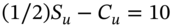 or
or  . Since the outcome at
  is the same whether the stock price goes ‘up’ or ‘down’, then for no risk-free arbitrage opportunities (see Equation (21.5)) we require
  , which we can solve to give
  .
.