CHAPTER 40
Pricing Fixed Income Options: Black's Model and MCS
Aims
- To show how Black's model provides closed-form solutions for the price of European options on T-bonds, on T-bond futures, on caps, floors, collars and on European swaptions.
- To price fixed income options using Monte Carlo simulation (MCS).
In previous chapters we discussed hedging/insurance using options on T-bonds and Eurodollar futures and how caps, floors, collars, and swaptions are used to hedge/insure interest sensitive assets and liabilities such as floating rate bank deposits and loans. In this chapter we concentrate on how to price some of these derivatives. To price fixed income derivatives we can use:
- Black's model which gives closed form solutions
- MCS under risk-neutral valuation (RNV)
- BOPM model with an interest rate lattice (tree)
- Equilibrium term structure approach.
Black's model assumes the price of the underlying asset in the options contract has a lognormal distribution, at maturity of the option. MCS generates a path for the short-rate and prices the derivative under RNV. The BOPM uses a lattice for the ‘short-rate’ of interest. The equilibrium yield curve approach assumes a specific stochastic process for the interest rate and solves mathematically for the derivatives price – the BOPM and the equilibrium yield curve approach are dealt with in Chapters 41 and 49, respectively.
40.1 BLACK'S MODEL: EUROPEAN OPTIONS
Black's (1976) model, which was originally used for pricing options on commodity futures can be adapted to give a closed-form solution for prices of European bond options, futures options, caps, floors, and European swaptions. The cash payout on an interest rate option may occur on the expiration date of the option, ![]() . But note that for some options the payoff
. But note that for some options the payoff![]() is determined at
is determined at ![]() , but the actual cash payout is delayed to
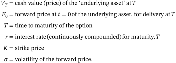
, but the actual cash payout is delayed to ![]() . We adopt the following notation:
. We adopt the following notation:
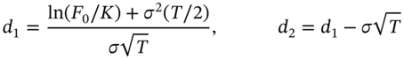
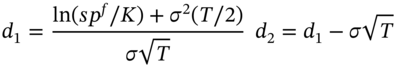
Black's model does not assume a GBM for the underlying but requires somewhat weaker assumptions namely, that at expiration ![]() is normally distributed with standard deviation of
is normally distributed with standard deviation of ![]() and
and ![]() , the forward price. If the European (fixed-income) option has a payoff, which is paid at
, the forward price. If the European (fixed-income) option has a payoff, which is paid at![]() , then Black's formulas for the call and put premia are:
, then Black's formulas for the call and put premia are:
If the option payoff is determined at ![]() , but the actual cash payment is delayed until T* then the above formulas for
, but the actual cash payment is delayed until T* then the above formulas for ![]() still apply (i.e. using
still apply (i.e. using ![]() ) but the discount factor is
) but the discount factor is ![]() (where
(where ![]() is the interest rate for maturity
is the interest rate for maturity ![]() ).
).
40.1.1 European Bond Option
For a European option on a T-bond, the futures price of the bond is given by ![]() where
where ![]() is the present value of the coupons on the T-bond, payable over the life of the option and
is the present value of the coupons on the T-bond, payable over the life of the option and ![]() is the current cash price of the bond. The volatility
is the current cash price of the bond. The volatility ![]() used in Black's model is for the forward bond price.
used in Black's model is for the forward bond price.
40.1.2 Caps and Floors
Consider a caplet on 90-day LIBOR on a notional principal ![]() with strike rate
with strike rate ![]() . The
. The ![]() and the caplet matures in
and the caplet matures in ![]() . If the out-turn 90-day LIBOR rate at maturity of the cap is
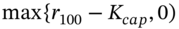
. If the out-turn 90-day LIBOR rate at maturity of the cap is ![]() the payoff at maturity is:
the payoff at maturity is:
The payoff is calculated at ![]() but is paid at
but is paid at ![]() . Note that
. Note that ![]() is continuously compounded, whereas
is continuously compounded, whereas ![]() and
and ![]() refer to simple annual rates. Assume
refer to simple annual rates. Assume ![]() is normally distributed with standard deviation
is normally distributed with standard deviation ![]() then:
then:
Invoice price of caplet that matures at  :
:
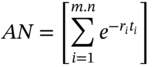
40.1.3 Caps
Suppose we have a cap on a notional principal of ![]() with
with ![]() -reset dates,
-reset dates, ![]() with the final payment at
with the final payment at ![]() . The tenor is the time between the reset dates (measured in years),
. The tenor is the time between the reset dates (measured in years), ![]() .
.
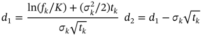
To price a cap, each caplet must be valued separately (see Equation 40.4) but this requires different forward volatilities ![]() for each caplet. However, in practice cap premia are often quoted using flat volatilities – that is,
for each caplet. However, in practice cap premia are often quoted using flat volatilities – that is, ![]() is assumed to be constant for all horizons
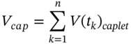
is assumed to be constant for all horizons ![]() . The invoice price of a cap is the sum of the caplet premia that comprise the cap.
. The invoice price of a cap is the sum of the caplet premia that comprise the cap.
40.1.4 Floorlet and Floors
The invoice price of a floorlet that matures at ![]() is:
is:
and the invoice price of a floor is the sum of the floorlet premia that make up the floor.
40.2 PRICING A CAPLET USING MCS
MCS can often provide a quick and conceptually easy method of valuing some fixed-income derivatives. For example, under RNV the price of a caplet is:
For example, consider pricing a caplet (on 90-day LIBOR) with a strike price ![]() and
and ![]() . To use MCS we need to generate a data series for the short-term LIBOR rate. Suppose we choose a discrete approximation to Vasicek's mean reverting model:
. To use MCS we need to generate a data series for the short-term LIBOR rate. Suppose we choose a discrete approximation to Vasicek's mean reverting model:
where ![]() – niid(0,1). The (mean) long-run interest rate might be
– niid(0,1). The (mean) long-run interest rate might be ![]() p.a. (0.03) and the rate of convergence,
p.a. (0.03) and the rate of convergence, ![]() . We take
. We take ![]() , so we divide 1 year into
, so we divide 1 year into ![]() time units. Assume that the current short rate is
time units. Assume that the current short rate is ![]() p.a. (0.04) and the notional principal in the caplet is
p.a. (0.04) and the notional principal in the caplet is ![]() . MCS involves the following steps:
. MCS involves the following steps:
- Generate
 observations on
  and calculate its average value,
- Calculate the payoff of the caplet at expiration =
- The price of caplet for the first Monte Carlo run is

- Repeat the above steps for
 runs of the MCS then:
(40.7)
runs of the MCS then:
(40.7)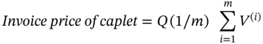
It is easy to see how this method can be applied to other interest rate derivatives discussed above. For example, the value of a cap using MCS is simply the sum of the MCS prices of the individual caplets (with different maturity dates and strikes).
Option premia calculated using MCS are dependent on the specific stochastic model chosen for the short rate. Hence estimation issues arise. But the option can be priced using MCSs with alternative stochastic processes for the interest rate – and the sensitivity of alternative MCS option premia to alternative stochastic processes can be assessed.
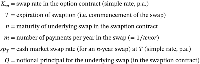
40.3 EUROPEAN SWAPTION: BLACK'S MODEL
A ‘pay-fixed, receive-floating’ swap is equivalent to being short a fixed rate bond and long a floating rate bond. A payer swaption is an option to enter into an interest rate swap at maturity of the option contract ![]() , to pay-fixed, receive-floating at an agreed swap rate
, to pay-fixed, receive-floating at an agreed swap rate ![]() , on a notional principal
, on a notional principal ![]() over the life of the swap. The underlying swap in the swaption contract begins at
over the life of the swap. The underlying swap in the swaption contract begins at ![]() and matures at
and matures at ![]() years. (A receiver swaption is an option to enter into a swap contract to receive-fixed, pay-floating at an agreed swap rate
years. (A receiver swaption is an option to enter into a swap contract to receive-fixed, pay-floating at an agreed swap rate ![]() .) We use the following notation (Figure 40.1) and assume the swap rate at
.) We use the following notation (Figure 40.1) and assume the swap rate at ![]() is lognormal:
is lognormal:
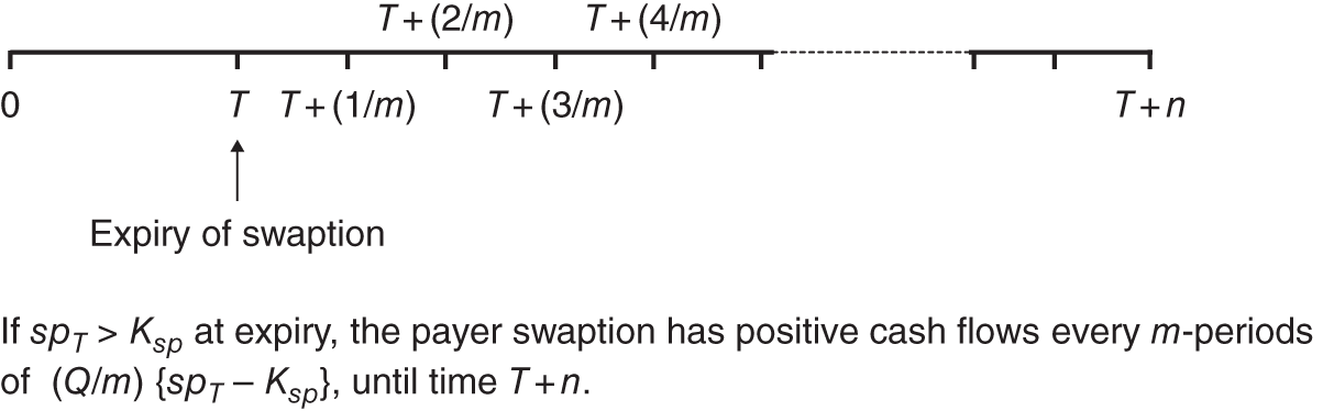
FIGURE 40.1 Payer swaption
A payer swaption gives rise to a series of cash flows at expiration:
which accrue at ![]() years from today (where
years from today (where ![]() ) – see Figure 40.1. The value today
) – see Figure 40.1. The value today ![]() , of any one of these cash flows received at time
, of any one of these cash flows received at time ![]() is given by Black's formula:
is given by Black's formula:

At ![]() we know the forward swap rate,
we know the forward swap rate, ![]() . A payer swaption comprises a series of cash flows, hence its value (invoice price) today, at
. A payer swaption comprises a series of cash flows, hence its value (invoice price) today, at ![]() is:
is:
![]() is the present value of an annuity of $1 paid at
is the present value of an annuity of $1 paid at ![]() over
over ![]() periods.
periods.
If we have a receiver swaption (i.e. receive-fixed, pay-floating) then the payoff is ![]() and the invoice price of the put is:
and the invoice price of the put is:
40.3.1 Limitations of Black's Formula
Black's model is widely used in practice because it provides a closed-form solution for European option premia on T-bonds (and T-bond futures), Eurocurrency futures and on swaps (i.e. swaptions). However, Black's model has its limitations. First, it is inconsistent to assume that at expiration of the option, the bond price, the bond futures price, the short rate, and the swap rate are all lognormally distributed.
Second, in reality a bond price or interest rates do not have a constant volatility over the life of the option but Black's formula assumes a constant volatility. For example, the volatility of the price of a bond approaches zero as the bond nears its maturity date. However, if the T-bond or T-bond futures option has a maturity T which is small relative to the ‘life’ of the underlying bond being delivered, then the constant volatility assumption may provide a reasonable approximation.
Note that Black's model only deals with European and not American or other ‘more exotic’ fixed income options. Some of the weaknesses of Black's model can be dealt with by using MCS – for example, we can incorporate stochastic volatility – but as we shall see in Chapter 41, the BOPM is also useful in pricing fixed income securities.
40.4 SUMMARY
- Black's (1976) model can be adapted to give a closed-form solution for pricing certain fixed-income options as long as we assume that at expiration, either interest rates or bond prices or futures prices are distributed lognormally. The latter cannot be true for all three ‘prices’ but this is often ignored in practice because of the tractability of Black's formula.
- Black's formula is used to price European options on T-bonds (and T-bond futures) as well as caps, floors, and swaptions.
- Monte Carlo simulation provides a flexible approach to pricing many types of fixed income options, including (some) path-dependent options. Of course, the resulting option prices will only be accurate if the stochastic process assumed for interest rates is a reasonable representation of their future behaviour. The robustness of the calculated MCS option premia can be assessed using alternative stochastic processes for interest rates.
EXERCISES
Question 1
Black's model can be applied to European options on T-bonds, T-bond futures, caps, floors, and swaptions. What key assumptions are required to apply Black's model?
Question 2
When pricing a caplet using MCS why do we not assume that the interest rate follows a geometric Brownian motion (GBM)?
Question 3
What are the key factors which determine the payoff at maturity from a 3-year payer swaption with notional principal Q, tenor of 90 days and a swap life of 2 years?
Question 4
Use Black's model to value a 6-month European put option on a 10-year bond with strike price ![]() . The current price of the 10-year bond is
. The current price of the 10-year bond is ![]() .
.
Present value of coupons on the bond (paid during the life of the option), ![]() . The 1-year interest rate
. The 1-year interest rate ![]() p.a. (continuously compounded). The bond's (forward price) volatility is 5% p.a.
p.a. (continuously compounded). The bond's (forward price) volatility is 5% p.a.
Show your calculations for ![]() , etc.
, etc.
Question 5
Today, using Black's model, on a ![]() option, the implied price volatility for an underlying bond which matures 10 years from today is
option, the implied price volatility for an underlying bond which matures 10 years from today is ![]() . Suppose this implied volatility
. Suppose this implied volatility ![]() is used today to price a
is used today to price a ![]() option (on the same 10-year bond). Would the option price for the
option (on the same 10-year bond). Would the option price for the ![]() option be too high or too low?
option be too high or too low?
Question 6
Use Black's model to calculate the price of a 9-month cap, on 90-day LIBOR, with strike ![]() (actual/360, day count) and principal
(actual/360, day count) and principal ![]() . The (interest-rate) volatility is
. The (interest-rate) volatility is ![]() p.a. and the 90-day forward rate (beginning in 9 months) is
p.a. and the 90-day forward rate (beginning in 9 months) is ![]() (simple rate, actual/360).
(simple rate, actual/360).
The yield curve is flat at ![]() p.a. (over 90 days, simple rate) so
p.a. (over 90 days, simple rate) so ![]() hence
hence ![]() , which gives
, which gives ![]() p.a. (continuously compounded).
p.a. (continuously compounded).
Show your calculations for ![]() , etc.
, etc.
Question 7
The underlying asset in a (T = 3-year) payer swaption with a strike of ![]() p.a. is an N = 4-year swap, with annual payments (tenor = 1 year) and principal Q = $100,000. The volatility of the 4-year (forward) swap rate,
p.a. is an N = 4-year swap, with annual payments (tenor = 1 year) and principal Q = $100,000. The volatility of the 4-year (forward) swap rate, ![]() p.a.
p.a.
The yield curve is currently flat at ![]() p.a. (continuous compounding). Forward rates at all maturities are 8% p.a. (continuous compounding) which gives a forward swap rate (simple rate) of
p.a. (continuous compounding). Forward rates at all maturities are 8% p.a. (continuous compounding) which gives a forward swap rate (simple rate) of ![]() . The volatility of the (4-year) forward swap rate,
. The volatility of the (4-year) forward swap rate, ![]() p.a.
p.a.
Show your calculations for ![]() , etc.
, etc.
NOTE
- 1 If
 is the continuously compounded rate and the yield curve is flat then the forward rate (simple rate, tenor = 180/360) is
 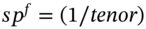 * (exp(r*tenor) – 1) = 4.04%.