CHAPTER 44
Value at Risk
Aims
- To explain the concept of value at risk (VaR).
- To measure VaR using the variance-covariance (VCV) approach.
- To outline methods used in forecasting volatility.
- To use backtesting to assess the accuracy of VaR forecasts.
- To outline the ‘Basel internal models’ approach in setting regulatory standards.
44.1 INTRODUCTION
Financial institutions, particularly large investment banks, hold positions in a wide variety of assets such as stocks, bonds, foreign exchange, as well as futures and options contracts. Because prices of these assets can move quickly and by large amounts, investment banks want to know what risk they are holding over the next 24 hours as well as over the next week or month. Once they know what their risk position is then they can either decide to maintain or reduce it or alternatively to hedge the risk – usually by using derivatives. Risk due to price changes is known as ‘market risk’ and measuring and monitoring changing market risk is the subject of this chapter.
For their own prudential reasons financial intermediaries need to measure the overall ‘dollar’ market risk of their portfolio, which is usually referred to as value at risk (VaR). In addition, the regulatory authorities use VaR to set minimum capital adequacy requirements for financial institutions. If a bank has a high VaR then the regulator may limit the amount of dividends paid to stockholders, so that the bank can increase its ‘capital’ via an increase in its retained profits. Alternatively, a bank can increase its ‘capital’ by issuing more stock to investors via a ‘seasoned offering’ (or ‘rights issue’ in the UK), which it often is reluctant to do because this dilutes the claims on future dividends of existing stockholders. The possibility of having to increase ‘bank capital’ using either of these methods is supposed to act as a deterrent to banks increasing their level of market risk to unacceptable levels.
The interaction between investment decisions and risk calculations is now absolutely central in managing mutual funds, hedge funds, pension funds, and a bank's marketable assets. The chief risk officer (CRO) in a financial institution has a key role in the risk management process.
In this chapter we examine how to measure market risk, mainly using stocks as our example. There are various ways to measure portfolio risk and we concentrate on the variance-covariance method (also called the delta-normal method). Since market risk varies over time we examine the accuracy of our forecast of VaR.
44.2 VALUE AT RISK (VAR)
In this section we use concepts from portfolio theory to provide us with a simple yet useful forecast of market risk, namely, value at risk – which is now the industry standard. Suppose you hold a portfolio of stocks. The return ![]() between today and tomorrow, is the capital gain or loss on the stocks (plus any cash payments such as dividends). However, dividend payments are announced in advance, so the source of uncertainty and risk over the next day (say) is mainly due to price changes. For simplicity, assume dividend payments are zero so that the return on a stock is1:
between today and tomorrow, is the capital gain or loss on the stocks (plus any cash payments such as dividends). However, dividend payments are announced in advance, so the source of uncertainty and risk over the next day (say) is mainly due to price changes. For simplicity, assume dividend payments are zero so that the return on a stock is1:
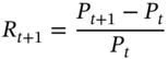
Measuring returns over 1 day allows us to determine daily VaR for a stock portfolio. Suppose you currently hold $3,030m in your stock portfolio and the CRO reports to the CEO of a bank, that over the next 24 hours (1 day) the VaR is $100m, at a 95% confidence level (also referred to as a 5% ‘left-tail’ value or 5th percentile). This implies that:
Given your current stock portfolio, there is a 95% chance (probability) that you will lose less than $100m over the next day (24 hrs).
Note that losing ‘less than’ $100m also means you might make gains on your portfolio – in fact there is a 50% chance you will make gains (if daily stock returns are normally distributed with a zero mean) – Figure 44.1.
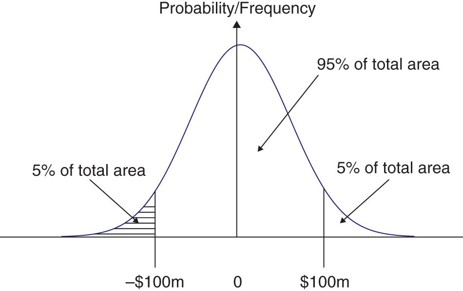
FIGURE 44.1 Normal distribution
Note that the risk officer is not saying you will lose less than $100m, only that there is a 95 out of 100 chance that you will lose less than $100m. So, as a concept VaR involves a specific probability or confidence level and a specific time horizon over which we measure risk. We cannot predict exactly how much you will lose (or gain) over any 24-hour period – since the world is risky – we can only provide a ‘best guess’ with a certain probability. This is not the only way we can express the daily VaR and an equivalent statement is:
Given your current stock portfolio then you expect to lose less than $100m (over any 24-hour period), in 19 out of the next 20 days.
You can see where ‘probability’ comes in, since ‘19 out of 20 days’ is equivalent to ‘95 days out of 100’, that is, 95% of the time. Hence, if you hold the $3,030m stock portfolio unchanged over the next 20 days, then on about 19 of those days you would lose less than $100m, hence:
If the daily portfolio VaR is $100m, at a 95% confidence level (5th percentile) then if you continue to hold your current stock portfolio, you expect to lose less than $100m in 19 of the next 20 days and to lose more than $100m on one day out of the next 20 days.
Note that even though the VaR concept is concerned with potential losses it is usually reported as a positive number. Much of the material discussed is based on the risk measurement methodology as set out in RiskMetricsTM (1996) which emanates from JPMorgan.
44.2.1 Measuring Risk
The riskiness of a single asset is summarised in the probability distribution of its returns. For daily stock returns the outcomes can take on many values and a convenient first assumption is that these outcomes are normally distributed. There is no single acceptable measure of the riskiness inherent in a particular statistical distribution, but for the normal distribution the standard deviation (or variance) is widely accepted as a measure of risk.
For normally distributed returns we can be 90% certain that the actual return will equal the expected return ![]() plus or minus
plus or minus ![]() (see Figure 44.2) where
(see Figure 44.2) where ![]() is the standard deviation of the returns. Put another way, we expect the actual return to be less than
is the standard deviation of the returns. Put another way, we expect the actual return to be less than![]() on 5% of occasions or greater than
on 5% of occasions or greater than ![]() , also on 5% of occasions (e.g. 1 time in 20).
, also on 5% of occasions (e.g. 1 time in 20).
FIGURE 44.2 Normal distribution
The mean daily return on a stock is small and close to zero. From a statistical point of view, there is so much ‘noise’ in daily returns (i.e. daily returns have a large standard deviation, relative to their mean return) so:
- when calculating daily VaR, we assume the mean return is zero.
- Hence,
 is a measure of the (per cent) ‘downside risk’ (at the 5th percentile).
If you hold a (net) position of ![]() in one asset (e.g. stock of AT&T), then the (dollar) VaR is:
in one asset (e.g. stock of AT&T), then the (dollar) VaR is:
which is a basic ‘building block’ for calculating the VaR of more complex portfolios.
A more direct approach to calculating the daily VaR is to note that the dollar change in value of the stock is ![]() , where
, where ![]() initial dollar holding in the stock,
initial dollar holding in the stock, ![]() daily return on the stock. It then follows directly that
daily return on the stock. It then follows directly that ![]() and hence the VaR at the 5th percentile is:
and hence the VaR at the 5th percentile is:
44.2.2 Are Daily Returns Normally Distributed?
Empirically, daily returns (i.e. daily price changes,![]() ) for exchange rates, long-term bond prices, and stock prices are all approximately normally distributed but they do deviate somewhat from normality, in the following ways:
) for exchange rates, long-term bond prices, and stock prices are all approximately normally distributed but they do deviate somewhat from normality, in the following ways:
- return distributions often have fatter tails than the normal distribution
- returns are negatively skewed (i.e. there are more observations in the left-tail than the right-tail).
In Figure 44.3 we show the histogram of daily returns using the S&P 500 index of US stocks – the mean daily return is very close to zero. The histogram is broadly ‘bell shape’, like the normal distribution. But the empirical distribution has a thinner peak than the normal distribution and there are a few more occurrences of extreme negative and positive returns than would be associated with the normal curve (i.e. the empirical histogram has fatter tails than the normal distribution) – this is excess kurtosis. In addition, the empirical distribution is reasonably symmetric so there is no appreciable negative or positive skew. In fact, for daily returns on most spot (cash market) assets it is probably a reasonable approximation to assume normality.
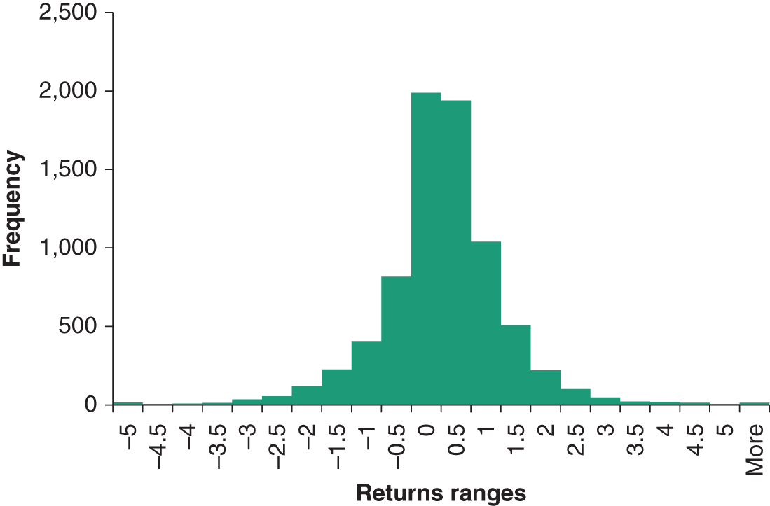
Figure 44.3 Daily returns S&P 500 (January 1990–March 2019)
44.2.3 Portfolio Risk
How can we measure the $-VaR of a portfolio of assets? First we present a ‘text book’ approach to this problem and then we use a more direct approach. Let's take two assets for simplicity – stocks of AT&T and Microsoft, in proportions (or ‘weights’) ¼ and ¾ respectively. The return ![]() on portfolio of stocks is:
on portfolio of stocks is:
The standard deviation of returns on the portfolio is given by the usual formula from portfolio theory (as found in standard text books):
where ![]() is the standard deviation of the return on stock-i and
is the standard deviation of the return on stock-i and ![]() is the correlation coefficient between the return on stock-1 (AT&T) and the return on stock-2 (Microsoft). So when we have a portfolio of stocks, consideration must be given to all the correlations between returns when calculating the portfolio standard deviation. (Note also that the term
is the correlation coefficient between the return on stock-1 (AT&T) and the return on stock-2 (Microsoft). So when we have a portfolio of stocks, consideration must be given to all the correlations between returns when calculating the portfolio standard deviation. (Note also that the term ![]() is the covariance between the two returns, usually written
is the covariance between the two returns, usually written ![]() .)
.)
In Equation (44.4)![]() is measured as a ‘per cent per day’ (expressed as a decimal) but the CEO of a bank is more interested in the dollar-VaR. By analogy with the single asset case the $-VaR for the portfolio is given by:
is measured as a ‘per cent per day’ (expressed as a decimal) but the CEO of a bank is more interested in the dollar-VaR. By analogy with the single asset case the $-VaR for the portfolio is given by:
where ![]() is the total amount invested in the stock portfolio. It is more convenient if the VaR calculation uses the dollar amount in each stock. If the initial dollar amounts held in each stock are
is the total amount invested in the stock portfolio. It is more convenient if the VaR calculation uses the dollar amount in each stock. If the initial dollar amounts held in each stock are ![]() and
and ![]() , then
, then ![]() and
and ![]() and
and ![]() . Substituting for
. Substituting for ![]() in (44.5):
in (44.5):
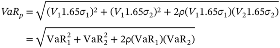
This is rather convenient since the dollar portfolio-VaR uses the individual dollar VaR's for each stock. If the dollar amounts held in each stock ![]() are positive, then the smaller the correlation between the two stock returns, the lower is
are positive, then the smaller the correlation between the two stock returns, the lower is ![]() . This is the usual diversification effect in portfolio theory. However, also note that if you have short-sold say $10m of stock-1 then
. This is the usual diversification effect in portfolio theory. However, also note that if you have short-sold say $10m of stock-1 then ![]() in Equation (44.6). So if stock-2 is held long then the larger is the positive correlation between the two stock returns, the smaller is portfolio risk and the VaR.
in Equation (44.6). So if stock-2 is held long then the larger is the positive correlation between the two stock returns, the smaller is portfolio risk and the VaR.
44.2.4 Worst-case VaR
Consider what would make ![]() a rather large number, indicating high portfolio risk. If stock returns are perfectly positively correlated
a rather large number, indicating high portfolio risk. If stock returns are perfectly positively correlated ![]() and you hold positive amounts in each stock
and you hold positive amounts in each stock ![]() , then this is a worst-case scenario, since there are no benefits from diversification. Thus the maximum value that
, then this is a worst-case scenario, since there are no benefits from diversification. Thus the maximum value that ![]() can take (for
can take (for ![]() ,
, ![]() ), known as the worst-case VaR, is given by setting
), known as the worst-case VaR, is given by setting ![]() in (44.6) which gives:
in (44.6) which gives:
Hence, the ‘worst-case VaR’ is simply the sum of the individual VaRs.2 In the real world it is unlikely that the correlation between the returns of two stocks like AT&T and Microsoft is +1, so your ‘best estimate of risk will usually be the diversified VaR’ given by Equation (44.6). However, in ‘crisis periods’ it is often the case that correlations increase, and the worst-case VaR provides a ‘high’ figure which may be representative of these crisis periods (e.g. during the 1987, 2000–1 and 2008 stock market crashes and the bond price meltdown of 1997). So, risk managers usually look at both the diversified-VaR and the worst-case VaR. This gives them a feel for what would happen if historic correlations did not stay the same but increased in a crisis period.
44.2.5 Two Assets
Using matrix algebra, Equation (44.6) can be succinctly written as:
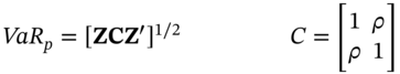
where ![]() is a row vector of the individual VaRs for each asset and
is a row vector of the individual VaRs for each asset and ![]() is the 2×2 correlation matrix.
is the 2×2 correlation matrix.
When we have more than n-assets, ![]() can be represented in exactly the same way but there are n entries in the
can be represented in exactly the same way but there are n entries in the ![]() -vector and the correlation matrix is
-vector and the correlation matrix is ![]() . Statisticians provide estimates of the next day's forecast of ‘volatilities’
. Statisticians provide estimates of the next day's forecast of ‘volatilities’ ![]() and correlation coefficients (in matrix C), while traders provide the dollar amounts
and correlation coefficients (in matrix C), while traders provide the dollar amounts ![]() they hold in each stock. So in practice, to calculate
they hold in each stock. So in practice, to calculate ![]() with n-stocks we need:
with n-stocks we need:
- the dollar position in each of the n-stocks
- forecasts of the daily standard deviation and correlations.3
As mentioned above, when reporting individual VaRs these are always taken as positive, even though they represent a potential loss (which conventionally has a negative sign). In calculating ![]() , the sign of the individual
, the sign of the individual ![]() must be incorporated in Z and if the stock is held long (i.e. you own it) then
must be incorporated in Z and if the stock is held long (i.e. you own it) then ![]() but if the stock has been short-sold then
but if the stock has been short-sold then ![]() . A simple example will clarify the issues involved.
. A simple example will clarify the issues involved.
44.2.6 VaR: Portfolio of Stocks
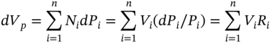
Now we calculate VaR using a more direct approach, which will be useful when we consider more complex portfolios (e.g. containing foreign assets and bonds) in the next chapter. For a portfolio of n-stocks, there is a linear relationship between the dollar change in the value of the portfolio ![]() and stock returns. Given
and stock returns. Given 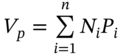 where
where ![]() ,
, ![]() , then:
, then:
where ![]() is the dollar amount in each stock and
is the dollar amount in each stock and ![]() is the (proportionate) return on stock-i. The above holds exactly for stocks and is a reasonable approximation for several other securities (e.g. the return on a foreign stock measured in domestic currency, the return on a bond, FRAs, FRNs, forwards, and futures). It follows directly from Equation (44.9) that the standard deviation of the dollar change in portfolio value is:
is the (proportionate) return on stock-i. The above holds exactly for stocks and is a reasonable approximation for several other securities (e.g. the return on a foreign stock measured in domestic currency, the return on a bond, FRAs, FRNs, forwards, and futures). It follows directly from Equation (44.9) that the standard deviation of the dollar change in portfolio value is:
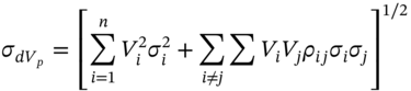
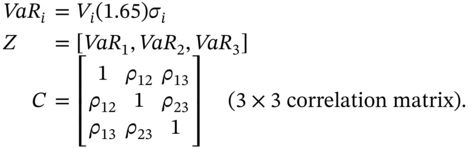
Equation (44.10) can be used to calculate the standard deviation of the dollar change in portfolio value regardless of the form of the distribution of stock returns. But the standard deviation alone does not allow us to determine the 5th percentile lower ‘cut-off’ value, unless we assume a specific distribution for asset returns. In particular, if we add the assumption of (multivariate) normally distributed asset returns, then the diversified-VaR at the 5th percentile is ![]() , which can be more compactly written (here, for
, which can be more compactly written (here, for ![]() assets):
assets):
where
The linearity and normality assumptions are crucial here. The change in portfolio value is sometimes perfectly consistent with linearity (e.g. for a stock portfolio) and where it is not, we often impose linearity as an approximation (i.e. we use a first order Taylor series expansion for the change in portfolio value). Note that if the relationship between ![]() and asset returns is highly non-linear (e.g. for stock options), then even if the returns of the underlying assets (stocks) are themselves normally distributed, the distribution of the change in the option's value will not be normally distributed. Hence, for a portfolio of options we cannot simply use the ‘
and asset returns is highly non-linear (e.g. for stock options), then even if the returns of the underlying assets (stocks) are themselves normally distributed, the distribution of the change in the option's value will not be normally distributed. Hence, for a portfolio of options we cannot simply use the ‘![]() ’ rule – we have to examine the complete distribution of outcomes, using MCS and other techniques.
’ rule – we have to examine the complete distribution of outcomes, using MCS and other techniques.
Providing we assume linearity and (multivariate) normality, all we need to calculate ![]() is the value of each asset holding
is the value of each asset holding ![]() and forecasts for the correlation coefficients and the return volatilities – hence it is known as the ‘variance-covariance’ (VCV) method. The worst-case VaR occurs when all the n-assets are assumed to be held long (i.e. all
and forecasts for the correlation coefficients and the return volatilities – hence it is known as the ‘variance-covariance’ (VCV) method. The worst-case VaR occurs when all the n-assets are assumed to be held long (i.e. all ![]() ) and all assets returns are perfectly positively correlated (hence C = the unit matrix where all elements are +1). Thus from (44.11):
) and all assets returns are perfectly positively correlated (hence C = the unit matrix where all elements are +1). Thus from (44.11):
The VaR for a portfolio of three stocks is given in Table 44.1. Each individual VaR is calculated as ![]() – this is in the fourth column. The worst-case VaR is simply the sum of the individual VaRs. The diversified VaR is calculated using the formula
– this is in the fourth column. The worst-case VaR is simply the sum of the individual VaRs. The diversified VaR is calculated using the formula ![]() . The diversified VaR is much smaller than the worst-case VaR because although all the correlation coefficients are positive, stock-2 has been short-sold (hence the ‘–10,000’ in the second column) and this ‘manufactures’ a negative correlation between its return and the returns on stocks 1 and 3. Hence there is a strong diversification effect and the (diversified) VaR at 783 is much less than the worst-case VaR of 1,996.
. The diversified VaR is much smaller than the worst-case VaR because although all the correlation coefficients are positive, stock-2 has been short-sold (hence the ‘–10,000’ in the second column) and this ‘manufactures’ a negative correlation between its return and the returns on stocks 1 and 3. Hence there is a strong diversification effect and the (diversified) VaR at 783 is much less than the worst-case VaR of 1,996.
TABLE 44.1 VaR, portfolio of three stocks
| Assets | Value | Std. dev. | VaR | Correlation matrix (= C) | |||
| 1 | 10,000 | 5.4180% | 894 | 1 | 0.962 | 0.403 | |
| 2 | –10,000 | 3.0424% | 502 | 0.902 | 1 | 0.61 | |
| 3 | 10,000 | 3.6363% | 600 | 0.403 | 0.61 | 1 | |
| Individual VaRs | 894 | −502 | 600 | ||||
| Worst case |
|||||||
| Diversified |
|||||||
44.3 FORECASTING VOLATILITY
It is clear from the above analysis that to calculate daily-VaR using the variance-covariance approach we need to forecast tomorrow's stock return volatility. A simple forecasting scheme is to assume that tomorrow's forecast of daily volatility is a simple moving average (SMA) of past squared returns ![]() , over the last 30 days (say):
, over the last 30 days (say):
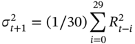
Note that in (44.12) we do not use the more usual term ![]() because we have assumed the mean daily return is zero. If today (= t) is Monday after the market has closed, then (44.12) gives a forecast of Tuesday's volatility based on the squared returns from Monday, last Friday's, Thursday's, etc., for the past 30 trading days. When ‘tomorrow’ arrives then on Tuesday, we make a new forecast. Now, our forecast for Wednesday includes Tuesday's, Monday's, etc. squared return (and we drop the final day's return from 31 days ago). Hence our forecast is continually updated as we ‘move through time’.
because we have assumed the mean daily return is zero. If today (= t) is Monday after the market has closed, then (44.12) gives a forecast of Tuesday's volatility based on the squared returns from Monday, last Friday's, Thursday's, etc., for the past 30 trading days. When ‘tomorrow’ arrives then on Tuesday, we make a new forecast. Now, our forecast for Wednesday includes Tuesday's, Monday's, etc. squared return (and we drop the final day's return from 31 days ago). Hence our forecast is continually updated as we ‘move through time’.
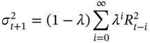
A problem with the SMA is that it gives equal weight (of 1/30) to all of the past 30 day's squared returns, when forecasting tomorrow's volatility. It seems more intuitive when forecasting ‘tomorrow’ to give relatively greater weight to what has happened in the recent past then in the more distant one. This can be achieved by using an exponentially weighted moving average (EWMA) forecast:
where ![]() is the daily return on the asset (with mean zero),
is the daily return on the asset (with mean zero), ![]() is a ‘weight’ lying between 0 and 1 (e.g.
is a ‘weight’ lying between 0 and 1 (e.g. ![]() ). The weights
). The weights ![]() decline exponentially, so this forecasting scheme is known as an EWMA model. For example, for
decline exponentially, so this forecasting scheme is known as an EWMA model. For example, for ![]() , the
, the ![]() weights decline as 0.94, 0.88, 0.83 ,…, etc. and squared returns which occur further in the past are given less weight in forecasting tomorrow's variance. Actually, the above equation can be written in a simpler form:
weights decline as 0.94, 0.88, 0.83 ,…, etc. and squared returns which occur further in the past are given less weight in forecasting tomorrow's variance. Actually, the above equation can be written in a simpler form:
Suppose you have 250 daily observations on squared returns ![]() . To start the recursive forecast using (44.13b) we might (arbitrarily) take a simple average of the first 30 observations on
. To start the recursive forecast using (44.13b) we might (arbitrarily) take a simple average of the first 30 observations on ![]() . If we denote this average as
. If we denote this average as ![]() then the forecast can be updated for day-31 using the ‘new’ value for
then the forecast can be updated for day-31 using the ‘new’ value for ![]() :
:
The forecast ![]() can then be updated daily until we get to day-100 after which the future values of
can then be updated daily until we get to day-100 after which the future values of ![]() ,
, ![]() etc. are independent of the initial value we used for
etc. are independent of the initial value we used for ![]() . As we have 250 days of historical data then we can continue the recursive forecast up to day-250. As additional information on daily returns becomes available our forecast of the variance (or standard deviation) changes as we move forward through time. It has been found that the EWMA forecasting equation gives better predictions than the SMA (based on the mean squared forecast errors).
. As we have 250 days of historical data then we can continue the recursive forecast up to day-250. As additional information on daily returns becomes available our forecast of the variance (or standard deviation) changes as we move forward through time. It has been found that the EWMA forecasting equation gives better predictions than the SMA (based on the mean squared forecast errors).
The above EWMA formula when applied to daily changes in the spot exchange rate is shown in Figure 44.4 and you can see how the EWMA forecasts move by quite substantial amounts and this will directly influence our changing daily forecasts of the VaR of a portfolio of foreign assets, which depends on the exchange rate.
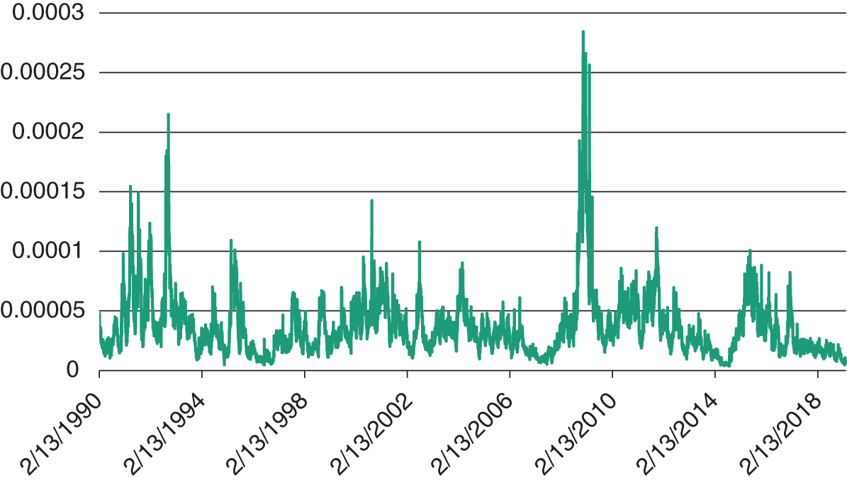
FIGURE 44.4 EWMA forecast – daily FX returns (Eurodollar)
Banks and financial institutions want to forecast the VaR not only over 1 day but also over other horizons such as a week or a month. However, it would be time consuming to calculate the many volatilities (not to mention correlations) required for these different horizons. Changes in weekly volatility are not the same as movements in daily volatility. However, if we assume daily (continuously compounded, log) returns are independent over time (and identically distributed) we can ‘scale them up’ to give a forecast of weekly or monthly volatility by using the ‘root T-rule’![]() . For iid returns, the standard deviation over T-days is:
. For iid returns, the standard deviation over T-days is:
So given our EWMA forecast of tomorrow's daily standard deviation ![]() we simply scale it up by
we simply scale it up by ![]() – the number of trading days over which we want to calculate the VaR.
– the number of trading days over which we want to calculate the VaR.
Forecasts for covariances use a similar EWMA scheme:
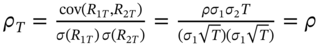
A forecast for the correlation coefficient is derived from the separate forecasts for variances and covariances4:
44.4 BACKTESTING
Forecasts of daily standard deviations and correlations for each stock and hence for the daily VaR will change from day to day (even when asset holdings remain unchanged). We want to assess whether our forecasts of daily portfolio-VaR are accurate at the 1st percentile. From the standard normal distribution the 1st percentile ‘cut off’ point is –2.33. The (changing) daily forecast of portfolio VaR at the 1st percentile is therefore ![]() . The historical out-turn for the actual daily (overnight) profit or loss (P/L) on the portfolio is
. The historical out-turn for the actual daily (overnight) profit or loss (P/L) on the portfolio is 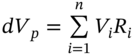 where
where ![]() are actual returns on successive days.5
are actual returns on successive days.5
In Figure 44.5, the rolling one-day-ahead forecasts ![]() are the two symmetric solid lines. The actual daily P/L on the portfolio
are the two symmetric solid lines. The actual daily P/L on the portfolio ![]() (assuming positions in the various assets are unchanged) are the ‘stars’. The actual P/L figures reflect the profit/loss that would have occurred if the initial $-position in each asset had been held over successive 24 hour periods over the past n = 600 days (say). The actual P/L does not reflect any position changes due to intraday trading.
(assuming positions in the various assets are unchanged) are the ‘stars’. The actual P/L figures reflect the profit/loss that would have occurred if the initial $-position in each asset had been held over successive 24 hour periods over the past n = 600 days (say). The actual P/L does not reflect any position changes due to intraday trading.
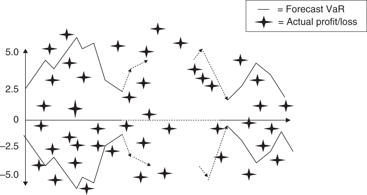
FIGURE 44.5 Backtesting
If the forecasts of ![]() (at the 1st percentile) are adequate then we should observe about 1 out of 100 ‘stars’ above the upper forecast-VaR solid line (and about 1 out of 100 below the lower solid line). If there are more than 1% of the ‘stars’ outside either of these lines, then our forecasts for
(at the 1st percentile) are adequate then we should observe about 1 out of 100 ‘stars’ above the upper forecast-VaR solid line (and about 1 out of 100 below the lower solid line). If there are more than 1% of the ‘stars’ outside either of these lines, then our forecasts for ![]() and
and ![]() and hence for the portfolio-
and hence for the portfolio-![]() , are an underestimate of the true portfolio risk. This procedure is known as backtesting.
, are an underestimate of the true portfolio risk. This procedure is known as backtesting.
In the hypothetical example in Figure 44.5 the actual losses over ![]() days, exceed the forecast-
days, exceed the forecast-![]() about 9 times out of 600 daily observations, when for an accurate VaR model we expect on average about
about 9 times out of 600 daily observations, when for an accurate VaR model we expect on average about ![]() outliers. Hence the VaR-forecast slightly overstates the potential losses, at the 1st percentile. If a financial regulator (e.g. Bank of England in the UK and the Fed in the USA) found many more than 9 out of 100 ‘exceedances’ (or ‘outliers’) then it might require a bank to hold more capital because of the poor performance of its risk model.
outliers. Hence the VaR-forecast slightly overstates the potential losses, at the 1st percentile. If a financial regulator (e.g. Bank of England in the UK and the Fed in the USA) found many more than 9 out of 100 ‘exceedances’ (or ‘outliers’) then it might require a bank to hold more capital because of the poor performance of its risk model.
Example44.4 tests whether the observed number of ‘outliers’ ![]() is consistent with the assumption of normally distributed returns and accurate forecasts of volatilities and correlations that lie behind the VaR forecasts.
is consistent with the assumption of normally distributed returns and accurate forecasts of volatilities and correlations that lie behind the VaR forecasts.
There are also ‘runs tests’ which check for independence in the VaR forecast outliers. If returns are independent over time as assumed in our VaR approach then any ‘outliers’ should appear in a random order over time. Put another way, we do not expect to see ‘bunching’ of outliers – that is, we should not observe five ‘outliers’, say, occurring in one specific week.
44.5 CAPITAL ADEQUACY
Financial firms (e.g. banks, mutual funds) hold positions in marketable assets and are therefore prone to losses. Prudential considerations imply that ‘capital’ (i.e. broadly speaking, the value of bank equity (stocks) held by investors in a bank plus cumulative retained profits) should be held as a ‘cushion’ against potential losses, otherwise the bank may become insolvent. The European Union, the Basel Committee (on Banking Supervision at the Bank for International Settlements, BIS) and the Federal Reserve Board (‘The Fed’) in the US have agreed that capital held by banks should reflect their market (and other) risks.
44.5.1 Basel Approach
The Basel ‘capital charge’ for market risk is based on the VaR of the bank's (market) portfolio: the higher the forecast portfolio VaR, the higher is the amount of capital it has to hold to meet regulatory requirements (see Finance Blog 44.1). But how high? This is determined by specific rules negotiated via the BIS, but with some discretion by the home regulator (e.g. in the UK this is the Financial Policy Committee [FPC], which is part of the Bank of England and this function is often part of a country's Central Bank responsibility).
Regulators also operate a green, yellow, and red, ‘traffic lights’ approach with more severe penalties, the worse the performance of a bank's VaR model when backtested. There is also more attention paid to a measure of risk known as ‘expected shortfall’, which is the (dollar) amount you expect to lose on average, given that your losses are greater than your VaR forecast. The figure for the expected shortfall is therefore greater than the figure for the VaR amount.
44.6 SUMMARY
- If the daily VaR for a portfolio of stocks is $10m, at a 95% confidence level (5th percentile) then you expect to lose no more than $10m in 5 out of the next 100 days and therefore you expect to lose more than $10m, on 5 days out of the next 100 days – assuming you hold an unchanged portfolio of stocks over the period.
- The (dollar) VaR for a stock portfolio is easily calculated using the variance-covariance method (VCV). The VCV approach assumes that each observed (daily) stock return is drawn independently from an identical distribution (i.e. same mean return and volatility) the return is normally distributed – in short, daily stock returns are assumed to be
 . In addition, daily returns across different stocks may be correlated – so returns are multivariate normal.
 - Forecasts of variances and covariances (correlations) of returns are often generated using the EWMA method.
- The
 -rule is often used for ‘scaling up’ daily volatility forecasts, in order to forecast VaR over longer horizons of up to 1 month (25 trading days) – this requires an assumption that daily returns are identically and independently distributed over time (but does not require that they are normally distributed).
 - Regulators check the accuracy of a bank's forecasts of portfolio-VaR by backtesting and set higher capital requirements when (a) the VaR forecast is high or (b) backtesting shows that the VaR forecasting model used is inaccurate.
EXERCISES
Question 1
Intuitively, why might you give more weight to recent movements in stock returns when forecasting tomorrow's volatility?
Question 2
Explain how you would assess whether your daily volatility forecasts for an individual stock return are accurate.
Question 3
A US investor holds $10m of AT&T shares and has short-sold $5m of Apple shares. Daily volatility of AT&T, ![]() and daily volatility of Apple,
and daily volatility of Apple, ![]() . The correlation between AT&T returns and Apple returns is –0.1. What is the $-VaR for this portfolio? What is the worst-case VaR?
. The correlation between AT&T returns and Apple returns is –0.1. What is the $-VaR for this portfolio? What is the worst-case VaR?
Question 4
You have a portfolio consisting of £10,000 in each of 3 assets, 1, 2, and 3. You have calculated the daily standard deviations to be 5.418%, 3.0424%, 3.6363%, respectively. The correlation between returns on asset-1 and asset-2 is 0.962, between asset-1 and asset-3 is 0.403, and between asset-2 and asset-3 is 0.610.
- What is the VaR for this portfolio?
- What is the worse-case VaR?
- What is the VaR if £10,000 of asset-2 is short-sold? Explain this result compared with the outcomes in (a) and (b).
Question 5
Your forecast of daily volatility, ![]() (1% per day). How might you forecast volatility over 25 (business) days? What assumptions are you making?
(1% per day). How might you forecast volatility over 25 (business) days? What assumptions are you making?
Question 6
Explain the step used in ‘backtesting’ forecasts of daily VaR at the 5th percentile. Assume you have $10m in each of two stocks and you have past daily data from 1 to T.
Question 7
Suppose the regulator for banks uses the 1st percentile to assess the VaR of a portfolio. What do you think the regulator would do if after backtesting the risk management system in your investment bank, found that actual losses exceeded your forecast-VaR losses 10 times in 175 forecasts?
NOTES
- 1 Alternatively, any dividend payments are added to the price at
 and then
  is the total return which equals the capital gain plus the dividend yield,
  .
. - 2 The worst-case VaR of Equation (44.7) also results from
 and
and  .
. - 3 If the number of assets in our portfolio is n, we have ‘n standard deviations’ and n(n – 1)/2 distinct correlations. For example, for
 that means 1,225 different correlation coefficients! Later we see how this very large number of correlations can be reduced by using the single index model (SIM).
 - 4 Also note that the correlation coefficient between returns over a T-day horizon is the same as the one-day correlation coefficient:
- 5 Usually, when we calculate the daily profit/loss
 , the values for
  are assumed to be held fixed each day at their initial values. This is the meaning of ‘an unchanged portfolio’. It is as if you start each successive day with
  held in each stock. In other words we do not ‘cumulatively update’ the value of each stock holding as returns change though time.
 - 6 Using the normal distribution as an approximation to the (‘true’) binomial distribution requires at least
 .
.