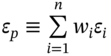
CHAPTER 45
VaR: Other Portfolios
Aims
- To show how we can reduce the number of computations required to calculate VaR, while still retaining the linearity assumption and hence allowing the use of the variance-covariance (VCV) method.
- To show how the single index model (SIM) is used to simplify the calculation of the VaR for a portfolio containing a large number of stocks.
- To demonstrate how a portfolio of foreign stocks can be viewed as equivalent to holding the foreign market index and the foreign currency. This allows calculation of VaR in the domestic currency, using the VCV method.
- To show how representing a coupon paying bond as a series of zero-coupon bonds allows calculation of the VaR using the VCV method, for portfolios containing many bonds with different cash flows and durations.
- To show how the VCV method can be used to calculate the (approximate) VaR for a portfolio of options.
45.1 SINGLE INDEX MODEL
We use the single index model (SIM) to show how the volatility of a well-diversified portfolio of stocks can be measured by the volatility of the market return (e.g. the S&P 500) and the portfolio beta. This substantially reduces the computational burden when calculating VaR because the large number of correlations between individual stock returns can be encapsulated in the portfolio beta, and therefore do not have to be estimated. But it must be remembered that the SIM requires several simplifying assumptions – most notably that specific random events that affect stock returns for one company are uncorrelated with random events which affect stock returns of another company.
45.1.1 Domestic Equity: SIM
Consider a portfolio consisting of n-stocks held in a specific country (e.g. USA). Forecasting the ![]() variances and particularly the
variances and particularly the ![]() correlations (covariances) across all stocks is computationally extremely burdensome, particularly for the covariance terms as there are so many of them. To ease the computational burden, we use the SIM since this allows all of the variances and covariances between returns to be subsumed into the n-asset betas (and a forecast for the variance of the market return). The SIM is:
correlations (covariances) across all stocks is computationally extremely burdensome, particularly for the covariance terms as there are so many of them. To ease the computational burden, we use the SIM since this allows all of the variances and covariances between returns to be subsumed into the n-asset betas (and a forecast for the variance of the market return). The SIM is:
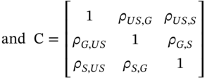
where ![]() is the return on stock-i,
is the return on stock-i, ![]() is the market return,
is the market return, ![]() is the beta of stock-i. The
is the beta of stock-i. The ![]() are (usually) assumed to be niid and in addition we make the crucial assumption that there is no contemporaneous correlation across the random error terms for different stocks (at time t),
are (usually) assumed to be niid and in addition we make the crucial assumption that there is no contemporaneous correlation across the random error terms for different stocks (at time t), ![]() . Hence, we assume that firm ‘specific risk’ (e.g. due to patent applications, IT failures, strikes, reputational effects, etc.) are uncorrelated across different firms. (Also,
. Hence, we assume that firm ‘specific risk’ (e.g. due to patent applications, IT failures, strikes, reputational effects, etc.) are uncorrelated across different firms. (Also, ![]() is independent of
is independent of ![]() .) An estimate of
.) An estimate of ![]() can be obtained either from a ‘risk measurement service’ (e.g. investment bank) or by running a time series regression of
can be obtained either from a ‘risk measurement service’ (e.g. investment bank) or by running a time series regression of ![]() on
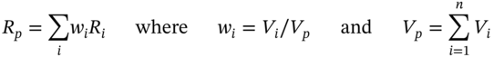
on ![]() (using say one year of daily returns data). Using (45.1) the return on a portfolio of n-stocks can be represented as:
(using say one year of daily returns data). Using (45.1) the return on a portfolio of n-stocks can be represented as:
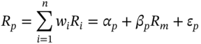
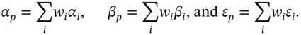
where  ,
,  ,
,  and
and ![]() is the proportion of total portfolio value held in each stock. From Equation (45.2), the portfolio return depends linearly on the market return (given the portfolio beta
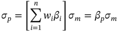
is the proportion of total portfolio value held in each stock. From Equation (45.2), the portfolio return depends linearly on the market return (given the portfolio beta ![]() ). It is easily shown that if
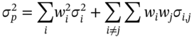
). It is easily shown that if ![]() , the variance of the portfolio return is:
, the variance of the portfolio return is:
where ![]() .
.
The specific risk of each stock ![]() can be ‘diversified away’ when stocks are held as part of a well-diversified portfolio (with small amounts held in each stock). Hence the term
can be ‘diversified away’ when stocks are held as part of a well-diversified portfolio (with small amounts held in each stock). Hence the term ![]() is small and can be ignored (see Appendix 45.B):
is small and can be ignored (see Appendix 45.B):
Thus when using the SIM we only require estimates of ![]() for the n-stocks and a forecast of
for the n-stocks and a forecast of ![]() , in order to calculate
, in order to calculate ![]() . We therefore dispense with the need to estimate n-values for the standard deviation of individual stock returns
. We therefore dispense with the need to estimate n-values for the standard deviation of individual stock returns ![]() and more importantly the n(n –1)/2 values for the correlation coefficients
and more importantly the n(n –1)/2 values for the correlation coefficients ![]() between all of the stock returns. This considerably reduces the computational burden of estimating the portfolio-VaR, which is given by:
between all of the stock returns. This considerably reduces the computational burden of estimating the portfolio-VaR, which is given by:
The SIM is a ‘factor model’ with only one factor, the market return ![]() . However, this approach could be extended within the VaR framework, by assuming several factors affect each stock return. For example, a widely used model is the so-called Fama–French three-factor model, where the return on any stock is determined by the market return
. However, this approach could be extended within the VaR framework, by assuming several factors affect each stock return. For example, a widely used model is the so-called Fama–French three-factor model, where the return on any stock is determined by the market return ![]() , the return on small (market cap) stocks minus large (market cap) stocks
, the return on small (market cap) stocks minus large (market cap) stocks ![]() and the return on high book-to-market minus low book-to-market stocks
and the return on high book-to-market minus low book-to-market stocks ![]() . Applying the SIM and the Fama–French three-factor model to each of the n-stock returns, implies that the forecast of portfolio variance
. Applying the SIM and the Fama–French three-factor model to each of the n-stock returns, implies that the forecast of portfolio variance ![]() only depends on estimates of the three factor betas, and forecasts of the three variances and six distinct covariances between the ‘three factors’ of the Fama–French model.
only depends on estimates of the three factor betas, and forecasts of the three variances and six distinct covariances between the ‘three factors’ of the Fama–French model.
45.1.2 Foreign Assets
How do we deal with exchange rate risk when calculating VaR for a portfolio that contains foreign assets? Suppose a US investor (Mr Trump) holds a €100m diversified portfolio in German stocks which exactly mirror movements in the German stock market index, the DAX. So, Trump's German stock portfolio has a beta of 1 with respect to the DAX market index. The dollar value of Mr Trump's German portfolio is subject to changes in the DAX and changes in ![]() , the Dollar-Euro spot FX-rate. In effect Mr Trump holds a two-asset portfolio, the foreign stock itself and the foreign currency. The percentage return on the German portfolio (in USD) is1:
, the Dollar-Euro spot FX-rate. In effect Mr Trump holds a two-asset portfolio, the foreign stock itself and the foreign currency. The percentage return on the German portfolio (in USD) is1:
where ![]() = return on the spot-exchange rate, that is
= return on the spot-exchange rate, that is ![]() . If stocks in the DAX fall at the same time as the euro depreciates against the US dollar, then Mr Trump would lose in USDs on both counts – a ‘double whammy’ of losses on the DAX itself plus losses when euros are converted into dollars. This is because after depreciation of the euro, for every euro that Mr Trump has in the DAX, he obtains fewer dollars.
. If stocks in the DAX fall at the same time as the euro depreciates against the US dollar, then Mr Trump would lose in USDs on both counts – a ‘double whammy’ of losses on the DAX itself plus losses when euros are converted into dollars. This is because after depreciation of the euro, for every euro that Mr Trump has in the DAX, he obtains fewer dollars.
Hence a positive correlation between the DAX index and the euro exchange rate increases the riskiness of the US investor's portfolio, measured in US dollars. Conversely, a negative correlation between the DAX and the euro exchange rate implies a lower dollar risk for Mr Trump's German stock portfolio.
To measure the dollar-VaR for a US investor with stocks held in the DAX we have to modify our previous VCV approach. First, because we are interested in the dollar-VaR we have to convert Trump's initial position in Euros, into USD. If Mr Trump has €100m invested in the DAX and the current Dollar-Euro spot FX rate is ![]() (USD per Euro), then the initial USD position is
(USD per Euro), then the initial USD position is ![]() . The key equation (see Appendix 45.A) is:
. The key equation (see Appendix 45.A) is:
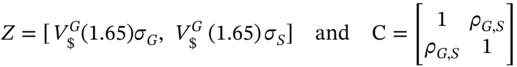
It follows directly that the dollar-VaR is then given by the usual formula:
where
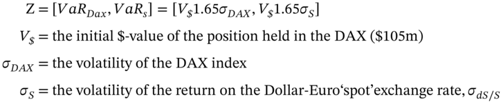
The Z-vector ‘contains’ the same $-value, ![]() for both the DAX and the FX position. This is because for a US investor, holding the DAX is equivalent to holding both
for both the DAX and the FX position. This is because for a US investor, holding the DAX is equivalent to holding both ![]() in the DAX plus
in the DAX plus ![]() in foreign exchange (euros). The correlation matrix C contains the correlation coefficient between the return on the DAX and the Euro-dollar spot exchange rate.
in foreign exchange (euros). The correlation matrix C contains the correlation coefficient between the return on the DAX and the Euro-dollar spot exchange rate.
45.1.3 German and US Stock Portfolios
Suppose (as above) a Mr Trump (a US investor) holds a portfolio of German stocks but the beta of the German stocks is ![]() and Mr Trump also holds a portfolio of US stocks with
and Mr Trump also holds a portfolio of US stocks with ![]() . Assume the US investor holds
. Assume the US investor holds ![]() dollars in US stocks and
dollars in US stocks and ![]() dollars in German stocks (that is,
dollars in German stocks (that is, ![]() , where
, where ![]() is the Euro-value of the German stock portfolio and
is the Euro-value of the German stock portfolio and ![]() is the current USD-Euro exchange rate). Assume the SIM holds within any single country, hence:
is the current USD-Euro exchange rate). Assume the SIM holds within any single country, hence:
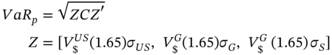
where ![]() = standard deviation of the S&P 500 US stock market index. The change in the dollar value of Mr Trump's portfolio is (approximately) linear in returns:
= standard deviation of the S&P 500 US stock market index. The change in the dollar value of Mr Trump's portfolio is (approximately) linear in returns:
where ![]() = return on German stock portfolio and
= return on German stock portfolio and ![]() , the proportionate change in the spot FX rate. The USD-VaR for this portfolio is:
, the proportionate change in the spot FX rate. The USD-VaR for this portfolio is:
This approach is easily extended to holding several foreign portfolios where for each foreign stock portfolio there are two entries in the Z vector – the VaR of the foreign stock portfolio and the VaR of the US-foreign currency, FX rate.
Suppose Mr Trump has a US stock portfolio as well as German and Brazilian stock portfolios (which are unhedged). Then there may still be some risk reduction (and hence a low portfolio VaR) if some of the spot FX rates have low (or negative) correlations with either the US-dollar exchange rate, or with stock market returns in different countries. If Mr Trump hedges his spot FX positions (using the forward market) then clearly any spot-FX volatilities and the correlation between spot FX-rates and foreign stock returns do not enter the calculation of VaR. But we cannot say unequivocally whether an unhedged or a FX-hedged ‘world portfolio’ has a lower risk – it depends on the interplay of the correlation coefficients in the two scenarios.
45.2 VaR FOR COUPON BONDS
Changes in bond prices and yields are not linearly related but we can use duration to give an approximate linear relationship. This then allows us to apply the variance-covariance approach to measure the VaR of a portfolio of coupon paying bonds. The easiest way to incorporate coupon paying bonds into the VCV approach is to note that for a portfolio of coupon paying bonds:
where  is the portfolio duration,
 ![]() = dollar amount in each bond and
= dollar amount in each bond and ![]() = total dollar amount in the portfolio of bonds,
= total dollar amount in the portfolio of bonds, ![]() . One problem with the above approach is that it assumes parallel shifts in the yield curve – that is, all spot yields move by the same absolute amount – which is encapsulated in the change in the (single) yield (to maturity)
. One problem with the above approach is that it assumes parallel shifts in the yield curve – that is, all spot yields move by the same absolute amount – which is encapsulated in the change in the (single) yield (to maturity) ![]() . Also the duration-approximation is not accurate for large changes in yields.
. Also the duration-approximation is not accurate for large changes in yields.
45.2.1 VaR: Non-parallel Shifts in the Yield Curve
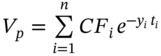
Can we improve on this approach and calculate the VaR for a portfolio of coupon paying bonds when there are non-parallel shifts in the yield curve? The way to do this is to consider a single coupon paying bond, with n-years to maturity, as a series of zero-coupon bonds. (This is extended to a portfolio of coupon paying bonds, below.) For a zero-coupon bond which has single cash flow ![]() at
at ![]() , the current value (price) is:
, the current value (price) is:
![]() = (continuously compounded) spot yield for period
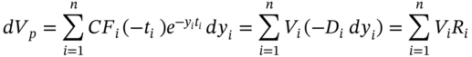
= (continuously compounded) spot yield for period ![]() . The proportionate change in value (price) of the zero-coupon bond is the ‘return’ on the bond, that is
. The proportionate change in value (price) of the zero-coupon bond is the ‘return’ on the bond, that is ![]() . Differentiating (45.11) we have a linear relationship between the return on the zero-coupon bond and the (absolute) change in yield:
. Differentiating (45.11) we have a linear relationship between the return on the zero-coupon bond and the (absolute) change in yield:
where for a zero-coupon bond ![]() (i.e. a zero-coupon bond's duration equals its maturity – measured in years). From (45.12):
(i.e. a zero-coupon bond's duration equals its maturity – measured in years). From (45.12):
A coupon paying bond is just a series of zero-coupon bonds and the value/price of a coupon bond with n-cash flows ![]() at time
at time ![]() is2:
is2:
Hence:
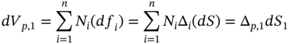
The dollar change in value of the coupon paying bond is (approximately) linear in the returns ![]() of its constituent zero-coupon bonds (for small changes in yields). We have ‘mapped’ the non-linear ‘yield-bond price relationship’ into an (approximate) linear framework. In addition, if we assume yield changes
of its constituent zero-coupon bonds (for small changes in yields). We have ‘mapped’ the non-linear ‘yield-bond price relationship’ into an (approximate) linear framework. In addition, if we assume yield changes ![]() are normally distributed, we can use Equation (45.14)3 to calculate the VaR (at the 5th percentile) for a coupon paying bond:
are normally distributed, we can use Equation (45.14)3 to calculate the VaR (at the 5th percentile) for a coupon paying bond:
where ![]() ,
, ![]() and C is the (n × n) correlation matrix of zero-coupon bond returns.
and C is the (n × n) correlation matrix of zero-coupon bond returns.
In general we do not forecast the volatility of bond returns ![]() directly, but instead forecast
directly, but instead forecast ![]() using the EWMA model. Then
using the EWMA model. Then ![]() provides a forecast of the standard deviation of (zero-coupon) bond returns for use in Equation (45.15). Similarly, we use the EWMA model to forecast the covariance
provides a forecast of the standard deviation of (zero-coupon) bond returns for use in Equation (45.15). Similarly, we use the EWMA model to forecast the covariance ![]() between changes in spot yields from which we obtain the correlation coefficients (for use in the correlation matrix
between changes in spot yields from which we obtain the correlation coefficients (for use in the correlation matrix ![]() ):
):
All of the above equations can be applied to a portfolio consisting of ![]() coupon paying bonds. The cash flows from the m-bonds at each time period
coupon paying bonds. The cash flows from the m-bonds at each time period ![]() are aggregated to give the total coupon payments at this date,
are aggregated to give the total coupon payments at this date,  . The current value of these coupons from all the bonds is then
 ![]() and the analysis follows as above.
and the analysis follows as above.
45.2.2 Mapping Cash Flows
A large investment bank may have coupon receipts on its bond portfolio virtually every week for the next 20–30 years. We cannot use current spot yields for every horizon ![]() over the next 30 years – there would be too many cash flows to deal with. To reduce the scale of the problem ‘standard vertices’ of say 1, 3, 6, and 12 months and 2, 3, 4, 5, 7, 9, 10, 15, 20, and 30 years, are used. All cash flows are ‘mapped’ onto these standard vertices and bond return volatilities
over the next 30 years – there would be too many cash flows to deal with. To reduce the scale of the problem ‘standard vertices’ of say 1, 3, 6, and 12 months and 2, 3, 4, 5, 7, 9, 10, 15, 20, and 30 years, are used. All cash flows are ‘mapped’ onto these standard vertices and bond return volatilities ![]() and correlations
and correlations ![]() are provided only for these chosen vertices.
are provided only for these chosen vertices.
For example, suppose an actual cash flow of $100m at ![]() (Figure 45.1) has to be apportioned between the standard vertices at
(Figure 45.1) has to be apportioned between the standard vertices at ![]() and
and ![]() . One approach (see Appendix 45.C) is to allocate cash flows to adjacent standard vertices to ensure that:
. One approach (see Appendix 45.C) is to allocate cash flows to adjacent standard vertices to ensure that:
- Total market value of the cash flows allocated to adjacent vertices (e.g. 5 and 7 years) equals the market value of the original cash flow (i.e. $100m at
 years).
 - The two cash flows at
 and
and  both have the same sign as the original cash flow.
 - The volatility of (present) value of the two cash flows at
 and
and  equal the volatility of the (present) value of the original cash flow at
  .
.
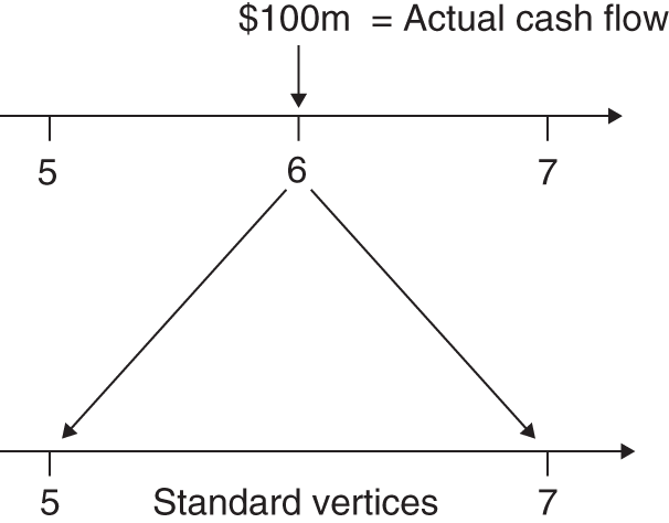
FIGURE 45.1 Mapping cash flows
45.2.3 Swaps
A pay-fixed, receive-floating interest rate swap is equivalent to a short position in a fixed rate bond and a long position in a FRN. The VaR for the fixed leg can therefore be analysed as a standard coupon paying bond. The value of the floating leg can be treated as a zero-coupon bond with a single known payment at the next payment date, discounted by the time to the next payment. Hence the VaR of the floating leg can also be calculated using the cash-flow mapping approach.
45.2.4 Principal Components Analysis
A useful alternative way of parsimoniously representing changes in say ![]() different spot yields is to use principal components analysis (PCA). PCA ‘represents’ the changes in all the
different spot yields is to use principal components analysis (PCA). PCA ‘represents’ the changes in all the ![]() spot yields by a few (usually about three) new variables called principal components (PCs).4 When computing the VaR of a bond portfolio we then use these three principal components, in place of the many
spot yields by a few (usually about three) new variables called principal components (PCs).4 When computing the VaR of a bond portfolio we then use these three principal components, in place of the many ![]() correlations between the original
correlations between the original ![]() spot yields.
spot yields.
PCA is a statistical technique which takes a ![]() matrix of changes in k-spot yields X, and seeks to ‘explain’ the movement in all these yields using just the three principal components, qi (i = 1, 2, 3). The q's are linear combinations (i.e. weighted averages) of the ‘raw’ spot rate data in the X-matrix:
matrix of changes in k-spot yields X, and seeks to ‘explain’ the movement in all these yields using just the three principal components, qi (i = 1, 2, 3). The q's are linear combinations (i.e. weighted averages) of the ‘raw’ spot rate data in the X-matrix:
where ci is an estimated constant. (It is in fact the eigenvalue corresponding to the largest eigenvector of the (X′X) matrix.) A major benefit of PCA is that the q's are orthogonal (uncorrelated) with each other and hence their correlation coefficients are zero (by construction).
It is generally found that about 95% of the variation in, say, 15 spot yields (e.g. for years 1, 2, 3, … 15) can be ‘empirically explained’ by about three PCs. The first PC is interpreted as representing parallel shifts in the yield curve, the second represents a twist in the yield curve, whereas the third (which explains the smallest proportion of the variation in the yield data) represents a ‘bowing’ in the yield curve (which occurs relatively infrequently). What is important for our VaR calculation is that the volatility of these 15 spot yields can be ‘linearly mapped’ into only three variables – the three PCs, ![]() . The three PCs are uncorrelated with each other and this considerably reduces the dimensionality of the VaR calculations.
. The three PCs are uncorrelated with each other and this considerably reduces the dimensionality of the VaR calculations.
45.3 VaR: OPTIONS
The VaR for options can be dealt with in the VCV framework if we are willing to use the linear approximation given by the option's delta. The change in value of a portfolio of call and put options on a specific stock (e.g. AT&T) but with different strikes and time to maturity, is given by the portfolio delta:
where ![]() is the change in the price of the call or put options (on AT&T stock). If the options on AT&T all have the same delta
is the change in the price of the call or put options (on AT&T stock). If the options on AT&T all have the same delta ![]() (i.e. same strike price and time to maturity) and there are
(i.e. same strike price and time to maturity) and there are ![]() options held, then the portfolio delta simplifies to
options held, then the portfolio delta simplifies to ![]() .
.
Now suppose we have options on two different stocks (Microsoft and AT&T) then:
The change in value of the options portfolio is (approximately) linear in the two stock returns and hence we can apply the standard VCV approach as in the following example.
Options prices are actually non-linear functions of the underlying asset (e.g. stock price). Hence, if changes in the stock prices are large, the delta approximation and VCV approach may provide a very poor measure of VaR for options portfolios. Superior techniques such as MCS and historical simulation are therefore the usual methods used to calculate VaR for portfolios containing options (see Chapter 46).
45.4 SUMMARY
- When using the VCV method, for a well-diversified stock portfolio containing n-stocks, use of the SIM simplifies the calculation. This is because the n-variances and n(n – 1)/2 correlations between the stock returns can be represented by the n-betas (that make up the portfolio beta) and the volatility of the market return. Therefore
 and
and 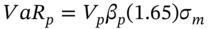 .
. - When a domestic investor holds a portfolio of foreign stocks she essentially holds a two-asset portfolio, the foreign stock portfolio and an equal amount in the foreign currency. The VCV approach can then be used to calculate the VaR.
- If we are willing to assume parallel shifts in the yield curve, the VaR of a portfolio of coupon-paying bonds can be reduced to the simple formula:
 .
. - For non-parallel shifts in the yield curve we can still apply the VCV approach to obtain the VaR for a portfolio of coupon-paying bonds (with n-cash flows). We model the coupon paying bonds as a set of zero-coupon bonds. The duration approximation allows the return on these zero-coupon bonds to be expressed as a linear function of changes in all of the spot yields. The VaR of the bond portfolio then depends on the volatility and correlations between all the spot yields at various maturities.
- In a large bond portfolio, coupon payments occur at many different time periods. To keep the VCV method tractable we have to ‘map’ these cash flows onto a smaller number of ‘standard’ time periods and calculate the VaR using only these standard time periods.
- The VaR for a portfolio of options can be analysed in the VCV framework using the options portfolio deltas. But this may be a poor approximation to the true VaR if the change in the underlying asset prices are large. This is because the true options prices are non-linear functions of the underlying asset prices and the delta approximation is only accurate for small changes in the underlying asset price.
APPENDIX 45.A: VaR FOR FOREIGN ASSETS
A US investor holds ![]() Euros in German stocks, which in USD is
Euros in German stocks, which in USD is ![]() , where
, where ![]() is the current Euro-USD spot exchange rate. The USD change in value of this portfolio is:
is the current Euro-USD spot exchange rate. The USD change in value of this portfolio is:
Let![]() be the (proportionate) change in the spot exchange rate (i.e. the return on foreign exchange). Substituting
be the (proportionate) change in the spot exchange rate (i.e. the return on foreign exchange). Substituting ![]() and rearranging:
and rearranging:
where we have ignored the cross product terms, which are small. In (45.A.2b) we see that the USD investor is effectively holding equal dollar amounts ![]() in German stocks and in the Euro-USD exchange rate. Hence it follows directly from (45.A.2):
in German stocks and in the Euro-USD exchange rate. Hence it follows directly from (45.A.2):
Therefore the USD-VaR for the US investor who holds the German portfolio is:
In addition, if we use the SIM then ![]() where
where ![]() is the portfolio-beta of the German stock portfolio and
is the portfolio-beta of the German stock portfolio and ![]() is the volatility of the German stock market index, the DAX.
is the volatility of the German stock market index, the DAX.
APPENDIX 45.B: SINGLE INDEX MODEL (SIM)
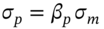
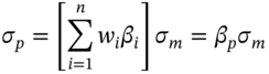
Using the single index model (SIM) we show that the standard deviation of a portfolio of n-stocks is:
where ![]() = portfolio standard deviation,
= portfolio standard deviation, ![]() = standard deviation of the market portfolio and
= standard deviation of the market portfolio and ![]() is the ‘beta’ of the stock portfolio. The SIM for each stock return is:
is the ‘beta’ of the stock portfolio. The SIM for each stock return is:
Assumptions:
It follows that :
The portfolio return and variance are:
The formula for portfolio variance requires n-variances and n(n – 1)/2 covariances. For example for ![]() this amounts to 11,325, inputs to estimate. To reduce the number of inputs required we utilize the SIM. Substituting from Equation (45.B.2) in (45.B.5a):
this amounts to 11,325, inputs to estimate. To reduce the number of inputs required we utilize the SIM. Substituting from Equation (45.B.2) in (45.B.5a):

Equation (45.B.7) may be interpreted as, ‘Total Portfolio Risk = Market Risk + Specific Risk’. Examining the specific risk term more closely and assuming ![]() , that is an equally weighted (i.e. well diversified) portfolio:
, that is an equally weighted (i.e. well diversified) portfolio:

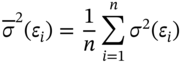
where we have used the key assumption of the SIM namely, ![]() . The average specific risk is defined as
. The average specific risk is defined as ![]() and as
and as ![]() this term goes to zero (n = 35 randomly selected stocks is usually sufficient to ensure this last term is relatively small). Hence under the SIM and assuming a well-diversified portfolio:
this term goes to zero (n = 35 randomly selected stocks is usually sufficient to ensure this last term is relatively small). Hence under the SIM and assuming a well-diversified portfolio:
A crucial assumption in the SIM is ![]() – the covariance of firm specific ‘random shocks’ to stock-i and stock-j are contemporaneously uncorrelated, across all stocks. This is reasonable for stocks in different sectors (e.g. oil and IT) but not for stocks in the same sector (e.g. Shell and BP). However, in a well-diversified portfolio even though there may be some small positive correlations between some
– the covariance of firm specific ‘random shocks’ to stock-i and stock-j are contemporaneously uncorrelated, across all stocks. This is reasonable for stocks in different sectors (e.g. oil and IT) but not for stocks in the same sector (e.g. Shell and BP). However, in a well-diversified portfolio even though there may be some small positive correlations between some ![]() and
and ![]() for daily returns, nevertheless portfolio specific risk still falls quite rapidly as
for daily returns, nevertheless portfolio specific risk still falls quite rapidly as ![]() increases and it is small relative to market (beta) risk. To see this note that from (45.B.8) that if
increases and it is small relative to market (beta) risk. To see this note that from (45.B.8) that if ![]() then:
then:
where ![]() is the average variance of the firm's specific risks and
is the average variance of the firm's specific risks and ![]() is the average covariance of the (contemporaneous) specific risks across firms:
is the average covariance of the (contemporaneous) specific risks across firms:
and
From (45.B.11a) the variance term goes to zero as n increases so for large ![]() , the variance of portfolio specific risk
, the variance of portfolio specific risk ![]() equals the average covariance between specific risks across different stocks,
equals the average covariance between specific risks across different stocks, ![]() . In a well-diversified portfolio where stocks are held across many different sectors (and countries), the average covariance of ‘specific risk’ across firms is likely to be small relative to market risk,
. In a well-diversified portfolio where stocks are held across many different sectors (and countries), the average covariance of ‘specific risk’ across firms is likely to be small relative to market risk, ![]() . Hence Equation (45.B.9) is a reasonable approximation. Of course, if our portfolio is not well diversified (e.g. we hold only energy stocks) then the assumption of the SIM that
. Hence Equation (45.B.9) is a reasonable approximation. Of course, if our portfolio is not well diversified (e.g. we hold only energy stocks) then the assumption of the SIM that ![]() will be incorrect and
will be incorrect and ![]() may be quite large. In this case our simplified expression for portfolio risk
may be quite large. In this case our simplified expression for portfolio risk ![]() ceases to hold and all the
ceases to hold and all the ![]() covariances
covariances ![]() are required for an accurate calculation of
are required for an accurate calculation of ![]() .
.
APPENDIX 45.C: CASH FLOW MAPPING
Mapping
A numerical example is the best way to illustrate this problem. Suppose we have an actual cash flow of $100m at ![]() years and we need to map this onto the ‘vertices’ at
years and we need to map this onto the ‘vertices’ at ![]() and
and ![]() (see Table 45.C.1).
(see Table 45.C.1).
TABLE 45.C.1 Data
| Time/Vertices | Yield | Price volatility = (1.65σ) | Correlation matrix |
| Year 5 |
|
|
1 0.99 |
| Year 7 |
|
|
0.99 1 |
To find the proportions of the actual cash flow of $100m at ![]() , which we should apportion to vertices
, which we should apportion to vertices ![]() and
and ![]() we proceed as follows:
we proceed as follows:
- The PV of the actual cash flow using
 is
is
- The yield at
 we take to be a linear interpolation of
  and
and 

- The volatility at t = 6 is a linear interpolation of
 and
and  :
:

- We apportion the cash flow at
 , between
  and
and  , to ensure positive cash flows at each vertex
  and that the volatility of
  is equal to
  :
(45.C.1)
:
(45.C.1)
We have estimates of
 (Table 45.C.1) and from Equation (45.C.2) we obtain two solutions
  or
or  (see below). We ignore the solution
  since it violates positive cash flows at both vertices (i.e.
  ). Hence for
  :(45.C.3)
 (45.C.4)
The results are summarised in Table 45.C.2.
TABLE 45.C.2 Mapping cash flow at ![]() to vertices at
to vertices at ![]() and
and ![]()
| Actual cash flow: $100m at 6 years | |||||||
| (1) Term |
(2) Actual cash flow |
(3) Yield |
(4) PV |
(5) Price vol. |
(6) Allocation weights, γ |
(7) Flows |
|
| Vertex 5 years | 5 years |
|
0.3 | 0.496 | $33.80m | ||
| Cash flow | 6 years | $100m |
|
$68.15m | 0.45 | ||
| Vertex 7 years | 7 years |
|
0.6 | 0.504 | $34.35m | ||
Solution for 
The left-hand side of (45.C.2) is a quadratic equation in ![]() of the form:
of the form:
with ![]() ,
, ![]() and
and ![]() . The solution of Equation 45.C.5 for
. The solution of Equation 45.C.5 for ![]() is:
is: ![]() which implies that 49.6 percent of the 6th year cash flow should be allocated to year-5.
which implies that 49.6 percent of the 6th year cash flow should be allocated to year-5.
EXERCISES
Question 1
Show how the single index model (SIM) can lead to considerable simplification when calculating the value at risk (VaR) over a 10-day horizon, for a portfolio of 20 domestic stocks with $10,000 in each stock. Clearly state any assumptions you make and their importance in determining the practical strengths and weaknesses of the SIM.
Question 2
What is ‘mapping’ and why is it useful in calculating the VaR for a portfolio consisting of coupon paying bonds?
Question 3
You are a US resident who holds a portfolio of UK stocks of £100m. The current USD/GBP exchange rate is 1.5 USD/GBP, the correlation between the return on the UK portfolio and the USD/GBP exchange rate is ![]() . The return on the FTSE All-Share index has a standard deviation of 1.896% per day and the volatility of the USD-GBP spot rate is
. The return on the FTSE All-Share index has a standard deviation of 1.896% per day and the volatility of the USD-GBP spot rate is ![]() per day. Using the variance-covariance VCV method calculate the daily US dollar VaR at the 5th percentile.
per day. Using the variance-covariance VCV method calculate the daily US dollar VaR at the 5th percentile.
Question 4
You are a US resident with €100m in the DAX-index and $100m face value in a US zero-coupon bond which matures in one year. The current spot FX rate is ![]() (USD/Euro) and the US spot interest rate is
(USD/Euro) and the US spot interest rate is ![]() . The daily standard deviations on the FX-rate, the DAX, and the US bond price are
. The daily standard deviations on the FX-rate, the DAX, and the US bond price are ![]() ,
, ![]() , and
, and ![]() , respectively. The correlation coefficients are
, respectively. The correlation coefficients are ![]() ,
, ![]() ,
, ![]() . Using the variance-covariance (VCV) method calculate the daily VaR of your portfolio (at the 5th percentile) and the worst-case VaR.
. Using the variance-covariance (VCV) method calculate the daily VaR of your portfolio (at the 5th percentile) and the worst-case VaR.
Question 5
A zero-coupon bond pays £1,000 in 2 years' time. You have the following information:
Current yield ![]() ., standard deviation of change in yield
., standard deviation of change in yield ![]() per day.
per day.
- Calculate the market value of the zero-coupon bond.
- Calculate the daily VaR for this bond (at the 5th percentile).
- Calculate the 10-day and 25-day VaR.
Question 6
You hold coupon bonds which pay $10,000 in 1 year's time and $110,000 in 2 years' time. The 1-year and 2-year spot yields are 3% p.a. and 4% p.a. respectively (continuously compounded). The volatility of the daily change in yields is ![]() (0.1% per day) and
(0.1% per day) and ![]() (0.2% per day).
(0.2% per day).
The correlation between the change in the 1-year and 2-year yields is 0.8.
Use the variance-covariance method (VCV) to calculate the daily VaR of this coupon bond (at the 5th percentile).
Question 7
A coupon paying bond has the following cash flow profile
| Year | 1 | 2 | 3 |
| Cash flow ($) | 400 | 450 | 500 |
| Spot rate (% p.a.) | 7.84 | 7.96 | 7.98 |
| Stdv of bond price changes (% per day) | 0.23 | 0.20 | 0.25 |
Spot yields are compound rates. The correlation between changes in the price (present value) of the 1-year, 2-year and 3-year cash-flows are ![]() ,
, ![]() , and
, and ![]() .
.
- Calculate the market value of each cash flow (i.e. price of the zero-coupon bonds).
- Calculate the (one day) VaR for each cash flow taken separately.
- Calculate the VaR of the coupon paying bond.
NOTES
- 1 This relationship is exact for continuously compounded returns but is an approximation for ‘standard’ returns.
- 2 Each cash flow
 consists of the sum of all the coupons
  or ‘coupons plus any repayments of principal’
  , hence,
  received at time
  , from the coupon-paying bond held. For T-bonds the par value
  is usually only paid at the maturity date but for corporate bonds with a ‘sinking fund’, the par value is often paid in instalments over the life of the bond – hence the use of
  for payment of part of the outstanding principal at
  .
. - 3 This can also be derived as follows.
 hence:
- 4 This idea is similar qualitatively in ‘reducing’ the number of covariances in a portfolio of n-stocks to a much smaller number of variances and covariances by using the SIM or with the Fama–French three-factor model, as discussed above.