CHAPTER 22
BOPM: Implementation
Aims
- To show how dynamic delta hedging can be used to price a (two-period) call option, using a portfolio comprising stocks and calls, which is risk-free over small intervals of time.
- To show how dynamic delta hedging is consistent with the no-arbitrage binomial pricing equation – the latter is a backward recursion that can be interpreted using risk-neutral valuation (RNV).
- To replicate the payoff to an option, using stocks and (risk-free) borrowing or lending (e.g. using a bank deposit/loan). This provides an alternative derivation of the binomial formula for options.
- To show that as each time-step in the binomial tree becomes smaller, the tree more closely approximates a continuous time process (Brownian motion) for the stock price – as used in the Black–Scholes approach. Hence, as we increase the number of time periods in the binomial tree, the option price calculated from the BOPM formula converges to the Black–Scholes price.
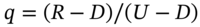
Using insights from RNV, we price a two-period call option using the BOPM without going through all the details involved in delta hedging and forming a ‘risk-free arbitrage portfolio’ – instead we price the option assuming RNV, using a ‘backward recursion’. This allows us to generalise the BOPM to many periods and to price many different types of option. We show that RNV is consistent with there being no arbitrage opportunities at any node in the binomial tree.
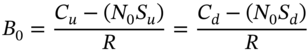
We demonstrate another method of pricing an option using a ‘replication portfolio’. We construct a portfolio consisting of stocks and risk-free borrowing or lending, which replicates the payoffs to the option. The price of the option must then equal the cost of setting up this replication portfolio, otherwise risk-free arbitrage profits can be made.
22.1 GENERALISING THE BOPM
We extend the BOPM (analysed in Chapter 21) and price a two-period call option with strike ![]() . The current stock price is
. The current stock price is ![]() , the one-period risk-free rate
, the one-period risk-free rate ![]() and
and ![]() the unknown call premium. As previously, we take
the unknown call premium. As previously, we take ![]() and
and ![]() which gives the stock price tree and values for a long call at expiration as indicated in Figure 22.1.
which gives the stock price tree and values for a long call at expiration as indicated in Figure 22.1.
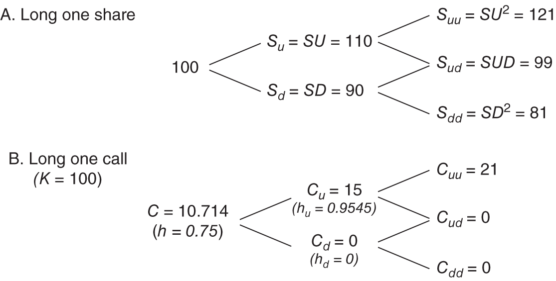
FIGURE 22.1 Two-period BOPM
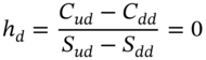
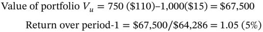
Because we create a risk-free hedge portfolio at each node of the binomial tree, we can invoke RNV and use ‘backward recursion’ to calculate ![]() from the known values of
from the known values of ![]() ,
, ![]() and
and ![]() . For example, from the two upper branches in Figure 22.1 we have:
. For example, from the two upper branches in Figure 22.1 we have:

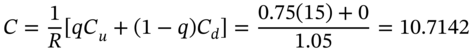
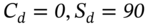
where ![]() . From the two lower branches:
. From the two lower branches:
We can now solve for ![]() , the call premium for this two-period case:
, the call premium for this two-period case:
Note that the call premium for the option with two periods to maturity has a higher value than our ‘identical’ option with one period to maturity, where we found ![]() (see
Chapter 21). Backward recursion (under RNV) is the easiest way of obtaining the option price. If we just consider European options, (where only the payoff at maturity determines the value of the option), then RNV provides a general formula for pricing calls and puts.
(see
Chapter 21). Backward recursion (under RNV) is the easiest way of obtaining the option price. If we just consider European options, (where only the payoff at maturity determines the value of the option), then RNV provides a general formula for pricing calls and puts.
22.1.1 Many Periods
Equations (22.1) and (22.2) give the values of ![]() and
and ![]() in terms of the final payoffs
in terms of the final payoffs ![]() ,
, ![]() and
and ![]() and if we substitute (22.1) and (22.2) in (22.3) we obtain:
and if we substitute (22.1) and (22.2) in (22.3) we obtain:
The European option price is equal to the expected value (using risk-neutral probabilities) of the option payoffs at maturity, discounted at the risk-free rate of interest.
The ‘2’ in the middle of Equation (22.4) represents the two possible paths to achieve the stock price ![]() (that is paths
(that is paths ![]() and
and ![]() ) and the ‘1's’ represent the single path to achieve either
) and the ‘1's’ represent the single path to achieve either ![]() or
or ![]() . We interpret
. We interpret![]() as the risk-neutral probability of an ‘up move’ for
as the risk-neutral probability of an ‘up move’ for ![]() and
and ![]() the probability of a ‘down move’. The (risk-neutral) probabilities of achieving the outcomes
the probability of a ‘down move’. The (risk-neutral) probabilities of achieving the outcomes ![]() ,
, ![]() or
or ![]() and
and ![]() are
are ![]() ,
, ![]() and
and ![]() , respectively. In general the number of possible paths to any final stock price are given by the binomial coefficients.
, respectively. In general the number of possible paths to any final stock price are given by the binomial coefficients.
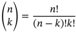
where ![]() is the number of periods in the binomial tree,
is the number of periods in the binomial tree, ![]() is the number of upward price movements and
is the number of upward price movements and ![]() and
and ![]() . Let's try out Equation (22.5) for
. Let's try out Equation (22.5) for ![]() :
:
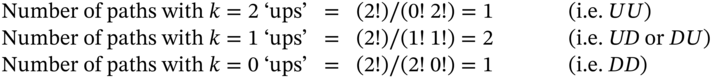
The reader might like to draw a tree with ![]() periods (with 8 possible final outcomes UUU, UUD, UDU, UDD, DUU, DUD, DDU, DDD), and verify that the number of possible paths to achieve
periods (with 8 possible final outcomes UUU, UUD, UDU, UDD, DUU, DUD, DDU, DDD), and verify that the number of possible paths to achieve ![]() ‘up’ moves is
‘up’ moves is 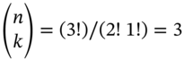 and these are UDD, DUD, and DDU. This can also be repeated using Equation (22.5) for
 ![]() or 3 ‘up’ moves. In general, over n-periods in the tree, the BOPM formula for a European call option is:
or 3 ‘up’ moves. In general, over n-periods in the tree, the BOPM formula for a European call option is:
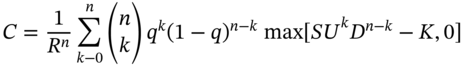
The probability of the stock price reaching the value ![]() after n-periods is
after n-periods is 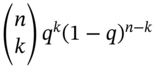 . Note that the term in square brackets in (22.6) is just another way of writing the payoffs at the final nodes. For example, for
 ![]() , these are:
, these are:
The price of a put option is also given by Equation (22.6) but with the term max[…] replaced by the sequence of put-option payoffs, namely ![]() . Equation (22.6) indicates that the price of an option depends on the strike price K, the underlying asset price S, the risk-free rate
. Equation (22.6) indicates that the price of an option depends on the strike price K, the underlying asset price S, the risk-free rate ![]() and the asset's volatility (which is determined by
and the asset's volatility (which is determined by ![]() and
and ![]() ), but it does not depend on the risk preferences of individuals or the ‘real-world’ probability of a price increase/decrease or the real world expected return on the stock. Below we show that as the number of nodes
), but it does not depend on the risk preferences of individuals or the ‘real-world’ probability of a price increase/decrease or the real world expected return on the stock. Below we show that as the number of nodes ![]() in the tree increases, we obtain a more accurate value for the option price and n > 30 generally gives reasonably accurate results for plain vanilla European options.
in the tree increases, we obtain a more accurate value for the option price and n > 30 generally gives reasonably accurate results for plain vanilla European options.
22.1.2 Where Do U and D Come From?
At ![]() ,
, ![]() , and
, and ![]() are known. Above we have shown that if we know
are known. Above we have shown that if we know ![]() and
and ![]() (and hence
(and hence ![]() ), then we can price an option by invoking RNV. It can be shown that the size of
), then we can price an option by invoking RNV. It can be shown that the size of ![]() and
and ![]() are determined by the actual real-world volatility of the stock return, and one method of achieving this is known as the Cox-Ross-Rubinstein (CRR) parameterisation:
are determined by the actual real-world volatility of the stock return, and one method of achieving this is known as the Cox-Ross-Rubinstein (CRR) parameterisation:
where ![]() the observed annual standard deviation of the (continuously compounded) stock return (decimal),
the observed annual standard deviation of the (continuously compounded) stock return (decimal), ![]() is the time to expiration of the option in years (or fraction of a year),
is the time to expiration of the option in years (or fraction of a year), ![]() is the number of steps chosen for the binomial tree so
is the number of steps chosen for the binomial tree so ![]() is a small interval of time. For example, if the expiration date of the option is at
is a small interval of time. For example, if the expiration date of the option is at ![]() year (3 months) and we choose a binomial tree with
year (3 months) and we choose a binomial tree with ![]() steps, then
steps, then ![]() years (i.e.
years (i.e. ![]() represents about 3 days out of a total of 365 calendar days per year).
represents about 3 days out of a total of 365 calendar days per year).
Given Equation (22.8), note that the ‘spread’ of the binomial lattice/tree (in percentage terms) at any two adjacent points (in a vertical direction) is ![]() , so the proportionate gap between
, so the proportionate gap between ![]() and
and ![]() (i.e.
(i.e. ![]() ) does depend directly on the ‘real world’ value of
) does depend directly on the ‘real world’ value of ![]() . Our particular choice for
. Our particular choice for ![]() and
and ![]() imposes symmetry that is
imposes symmetry that is ![]() but it can be shown that this is not restrictive if our aim is to construct a ‘risk-neutral’ lattice. Note also that when
but it can be shown that this is not restrictive if our aim is to construct a ‘risk-neutral’ lattice. Note also that when ![]() , the nodes
, the nodes ![]() and
and ![]() both have a value equal to
both have a value equal to ![]() and the lattice recombines. For example, if
and the lattice recombines. For example, if ![]() (at
(at ![]() ) is 100 it will also be 100 in the middle node at
) is 100 it will also be 100 in the middle node at ![]() . Finally, note that
. Finally, note that ![]() and
and ![]() do not depend on the real world expected return on the stock and hence neither does the option premium – this is RNV again.
do not depend on the real world expected return on the stock and hence neither does the option premium – this is RNV again.
We now have a very useful method of pricing a European call option (say), using RNV and backward recursion through the binomial tree:
- Choose
 > 30 and divide the time to maturity
  (in years) of the call option into small time intervals each representing
  (years).
 - If
 (decimal) is the (annual) continuously compounded interest rate then
  .
. - Construct the tree for the stock price using
 and
and  – this ensures the volatility of the stock return mimics its real world volatility.1
 - Calculate the possible final payoffs, max[0,
 ] at
] at  for the call option.
 - Use
 to calculate the expected payoffs for the call – this is RNV.
 - Undertake backward recursion through the tree, discounting the option values at the risk-free rate each period (this is RNV again), to finally obtain the option price at
 .
.
Although the above recursive method is very useful, it is worth remembering that the reason it works is because ‘behind the scenes’, at each node of the tree, we are implicitly assuming options traders are forming a risk-free delta-hedged portfolio so that no arbitrage profits are possible at any node – this is examined further in Appendix 22.
The option price will change as the stock price, stock return volatility, interest rate or the time to maturity change over time. We can calculate the (approximate) change in the price of the option using the option's ‘Greeks’ which include not only delta but the option's gamma, vega, theta, and rho. Calculation of the Greeks for the BOPM is explained in Chapter 28.
22.2 REPLICATION PORTFOLIO
22.2.1 Replicating a Long Call: One-period BOPM
In our original example, we priced the (one-period) call option by establishing a risk-free portfolio consisting of a written call and a long position in ‘delta’ stocks. We can also price the call by establishing a synthetic call or a replication portfolio for the call, using stocks and the risk-free asset. We combine stocks and the risk-free asset at ![]() into a ‘replication portfolio’ which gives exactly the same payoffs as the call
into a ‘replication portfolio’ which gives exactly the same payoffs as the call ![]() ,
, ![]() at
at ![]() . Because our ‘replication portfolio’ has the same payoff as the call (at
. Because our ‘replication portfolio’ has the same payoff as the call (at ![]() = 1), then the price of the call must equal the cost of setting up the ‘replication portfolio’ (at
= 1), then the price of the call must equal the cost of setting up the ‘replication portfolio’ (at ![]() = 0) – otherwise risk-free arbitrage profits are possible.
= 0) – otherwise risk-free arbitrage profits are possible.
Consider purchasing ![]() stocks at a price
stocks at a price ![]() and buying
and buying ![]() of risk-free (zero-coupon) bonds with a return
of risk-free (zero-coupon) bonds with a return ![]() – see Figure 22.2. When
– see Figure 22.2. When ![]() this implies a bond purchase (lending money) and
this implies a bond purchase (lending money) and ![]() implies issuing bonds (borrowing money). Hence,
implies issuing bonds (borrowing money). Hence, ![]() could just as easily be the amount borrowed in the form of a bank loan and
could just as easily be the amount borrowed in the form of a bank loan and ![]() , represents the amount placed in a bank deposit.
, represents the amount placed in a bank deposit.
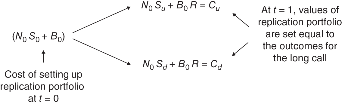
FIGURE 22.2 Replication portfolio
Replication Portfolio-A: Stocks plus Bonds
At ![]() , portfolio-A is worth either
, portfolio-A is worth either ![]() or
or ![]() and to replicate the payoff from a long call, we set these two values equal to
and to replicate the payoff from a long call, we set these two values equal to ![]() and
and ![]() , respectively:
, respectively:
Subtracting Equation (22.10b) from (22.10a) gives:
Substituting ![]() from Equation (22.11) into Equation (22.12) and using
from Equation (22.11) into Equation (22.12) and using ![]() ,
, ![]() :
:
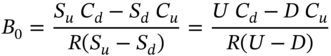
It is easy to see that the two expressions for ![]() in Equation (22.12) are equal by noting that they imply
in Equation (22.12) are equal by noting that they imply ![]() and given the definition of
and given the definition of ![]() in (22.11) these two expressions must be equal. As the portfolio of
in (22.11) these two expressions must be equal. As the portfolio of ![]() stocks and
stocks and ![]() (dollars) bonds is constructed to replicate the payoff of the call option at
(dollars) bonds is constructed to replicate the payoff of the call option at ![]() , then the call premium
, then the call premium ![]() (at time
(at time ![]() ) must equal the cost of the replication portfolio at
) must equal the cost of the replication portfolio at ![]() (otherwise arbitrage profits could be made):
(otherwise arbitrage profits could be made):
Substituting in (22.14) for ![]() from (22.11) and for
from (22.11) and for ![]() from (22.13), then after some manipulation we obtain:
from (22.13), then after some manipulation we obtain:
where ![]() . The number of stocks
. The number of stocks ![]() in Equation (22.11) required to replicate the payoffs of the call, is the hedge ratio
in Equation (22.11) required to replicate the payoffs of the call, is the hedge ratio ![]() in our earlier derivation.
in our earlier derivation.
22.2.2 Replicating a Long Call: Two-period BOPM
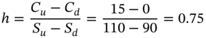
Now we use this approach to replicate the option values in a two-period lattice using stocks and the risk-free asset. Consider what is happening at ![]() (Figure 22.1). From (22.11) and (22.12) we have:
(Figure 22.1). From (22.11) and (22.12) we have:
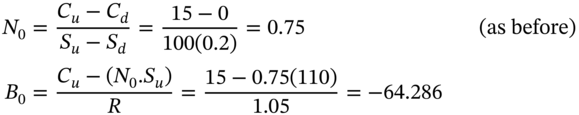
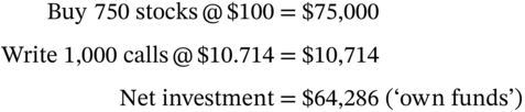
Note that here we are replicating the payoff of the long call (at ![]() ) with a long position in 0.75 of stocks and a short position in the bond (i.e. borrowing cash). At
) with a long position in 0.75 of stocks and a short position in the bond (i.e. borrowing cash). At ![]() the replication portfolio consists of borrowing $64.286 and purchasing $75 of stocks
the replication portfolio consists of borrowing $64.286 and purchasing $75 of stocks ![]() . This is a net investment of $10.714 which, not surprisingly, we have earlier found is the value of the option premium
. This is a net investment of $10.714 which, not surprisingly, we have earlier found is the value of the option premium ![]() (at
(at ![]() ) for a two-period call. The outcome in the ‘up’ and ‘down’ nodes for our ‘replication portfolio’ are:
) for a two-period call. The outcome in the ‘up’ and ‘down’ nodes for our ‘replication portfolio’ are:

which, of course, are the outcomes for the value of the call, ![]() , and
, and ![]() at the first two nodes. We now rebalance our replication portfolio so at the
at the first two nodes. We now rebalance our replication portfolio so at the ![]() -node:
-node:
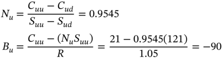
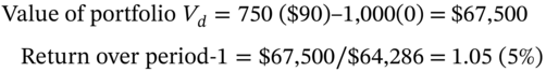
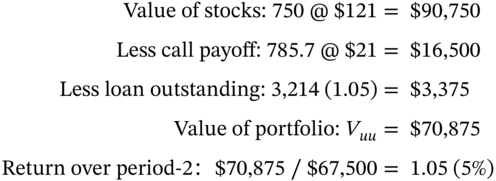
The reason for borrowing $90 at node U is that you must increase the number of stocks by (0.9545 – 0.75) = 0.2045 at a price of $110 per stock, giving a total cost of $22.5, which when added to your existing debt of 67.5 brings your debt to $90. The outcomes for the replication portfolio when moving from the U-node to the nodes UU and UD are:
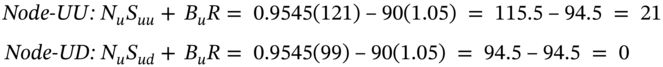
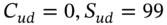
Again we have replicated the value of the call at these two nodes (see Figure 22.2). Finally, consider the D-node. Here ![]() and the replication portfolio consists of zero stocks and is entirely composed of bonds
and the replication portfolio consists of zero stocks and is entirely composed of bonds ![]() but because
but because ![]() (Figure 22.1), we hold no bonds at the D-node. The replication portfolio at node-D is therefore worth zero – but this exactly replicates the value of the call at the nodes
(Figure 22.1), we hold no bonds at the D-node. The replication portfolio at node-D is therefore worth zero – but this exactly replicates the value of the call at the nodes ![]() and
and ![]() (Figure 22.1).
(Figure 22.1).
Naturally, we obtain the same BOPM formula for the price of the call using either the ‘replication portfolio’ of stocks plus bonds or by using our earlier ‘delta hedge’ risk-free portfolio.
22.3 BOPM TO BLACK–SCHOLES
By increasing the number of steps n, in the binomial tree and seeing what happens to the option price in the BOPM, we obtain some insight into the Black–Scholes pricing formula for European options. As we increase the number of steps we are also shortening the time interval between each node in the binomial tree ![]() , so the BOPM becomes ‘more like’ the Black–Scholes approach, which uses continuous time mathematics, and the option price given by the BOPM formula converges towards the Black–Scholes price. Suppose we have:
, so the BOPM becomes ‘more like’ the Black–Scholes approach, which uses continuous time mathematics, and the option price given by the BOPM formula converges towards the Black–Scholes price. Suppose we have:
then the Black–Scholes formula gives a call premium ![]() . To translate these inputs into the BOPM we use
. To translate these inputs into the BOPM we use ![]() where
where ![]() is the number of steps in the binomial tree. We then calculate
is the number of steps in the binomial tree. We then calculate ![]() ,
, ![]() and
and ![]() as follows:
as follows:
For example, for ![]() we have:
we have:
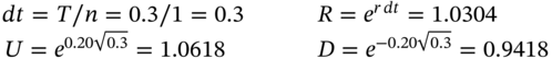
The call premium given by the BOPM using only one time-step is:
where ![]() ,
, ![]() ,
, ![]() . For
. For ![]() then we have
then we have ![]() which is not particularly close to the Black–Scholes value
which is not particularly close to the Black–Scholes value ![]() .
.
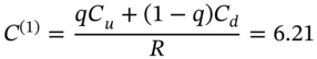
However, as we apply the recursive binomial Equation (22.6) for ![]() , etc. and dt = T/n, the binomial call price for
, etc. and dt = T/n, the binomial call price for ![]() is
is ![]() , which is close to the Black–Scholes value of
, which is close to the Black–Scholes value of ![]() – see Figure 22.3. In general, for plain vanilla European options (but not necessarily for complex exotic options) choosing
– see Figure 22.3. In general, for plain vanilla European options (but not necessarily for complex exotic options) choosing ![]() in the BOPM gives reasonably accurate results for the option price. The CRR parameterisation oscillates between over- and under-approximations (which are approximately symmetric) and which gradually dampen as the number of steps in the tree increases. The average of these over- and under-approximations converges rapidly towards the Black–Scholes price – for example, using only
in the BOPM gives reasonably accurate results for the option price. The CRR parameterisation oscillates between over- and under-approximations (which are approximately symmetric) and which gradually dampen as the number of steps in the tree increases. The average of these over- and under-approximations converges rapidly towards the Black–Scholes price – for example, using only ![]() steps in the binomial tree we have
steps in the binomial tree we have ![]() and
and ![]() and the average of the two is 5.3518, which is very close to
and the average of the two is 5.3518, which is very close to ![]() .
.
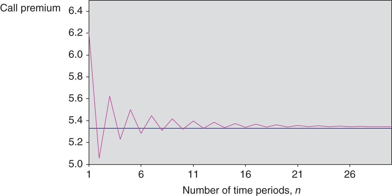
FIGURE 22.3 Call premium – BOPM and Black–Scholes
Of course, one problem with a numerical method like the BOPM is that it may not converge quickly and the solution can ‘bounce around’ the ‘correct’ option price given by Black–Scholes. This is the price you pay for the flexibility of the binomial approach. The option premium from the BOPM approaches that given by the Black–Scholes formula, as the number of steps increases (i.e. ![]() and hence
and hence ![]() ). The ‘up–down’ lattice of the BOPM then has many nodes and there are many possible paths the stock price could take (e.g. for just three nodes you can have eight possible paths (
). The ‘up–down’ lattice of the BOPM then has many nodes and there are many possible paths the stock price could take (e.g. for just three nodes you can have eight possible paths (![]() etc. – see below)). Hence as
etc. – see below)). Hence as ![]() the BOPM lattice approximates the geometric Brownian motion used by Black, Scholes and Merton in deriving the pricing formulas for European options.
the BOPM lattice approximates the geometric Brownian motion used by Black, Scholes and Merton in deriving the pricing formulas for European options.
Also notice that when the number of nodes in the binomial tree increases, the possible outcomes for stock prices in the final period (T) begin to look more like a ‘normal curve’. For example, with a probability of ![]() for an ‘up’ move,
for an ‘up’ move, ![]() ,
, ![]() and for
and for ![]() nodes the outcomes and probabilities are:
nodes the outcomes and probabilities are:
| Path | Probability | Final stock prices |
| UUU | 1/8 |
|
| UUD,DUU,UDU | 3/8 |
|
| UDD,DDU,DUD | 3/8 |
|
| DDD | 1/8 |
|
If the final stock prices are plotted in a histogram it looks (slightly) more like a ‘normal curve’ than if we just had ![]() with two outcomes 110 and 90 (each with probability of
with two outcomes 110 and 90 (each with probability of ![]() ). This is because for
). This is because for ![]() the ‘extreme’
the ‘extreme’ ![]() and
and ![]() outcomes each only occur 1/8th of the time but the central portion of the histogram for the paths with a one-up move or a one-down move, each occur 3/8ths of the time. In fact, as the number of nodes n increases (i.e. the time period between each node gets smaller) the ‘histogram’ for the final stock prices in the BOPM does approach a ‘normal curve’ – which is the assumption used in deriving the Black–Scholes formula.2
outcomes each only occur 1/8th of the time but the central portion of the histogram for the paths with a one-up move or a one-down move, each occur 3/8ths of the time. In fact, as the number of nodes n increases (i.e. the time period between each node gets smaller) the ‘histogram’ for the final stock prices in the BOPM does approach a ‘normal curve’ – which is the assumption used in deriving the Black–Scholes formula.2
22.4 SUMMARY
- RNV provides a way of obtaining the BOPM formula for option premia using backward recursion, which considerably simplifies the calculations. But behind this approach is the assumption that options traders are able to undertake dynamic delta hedging to eliminate any risk-free arbitrage profits.
- For European options, the BOPM is a backward recursion starting with the option payoffs at maturity
 , then calculating the expected value of the option at each node in the tree using risk-neutral probabilities and discounting these payoffs using the risk-free rate. Repeating this procedure as you move backwards through the tree, gives the ‘correct’ or ‘no-arbitrage’ option price.
 - The BOPM formula for the option premium can also be derived by replicating the payoffs to the option, using stocks and risk-free borrowing or lending (i.e. using either a risk-free bond or bank deposit/loan).
- In the BOPM the ‘size’ of the ‘up’
 and ‘down’
 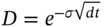 movements in the stock price depend on the ‘real world’ volatility of the stock return – and via
  in the BOPM, the option price depends on the volatility of the stock return.
 - The European option premium given by the BOPM, converges towards the Black–Scholes price, as the number of steps
 in the binomial tree increases (so each time-step in the tree represents a smaller interval of time).
 - The BOPM is a numerical technique, so it may suffer from convergence problems and only gives an approximation to the ‘true price’ – but it is a very flexible method which can be used to price exotic options.
APPENDIX 22: DELTA HEDGING AND ARBITRAGE
Given values for the call option determined by RNV in the two-period BOPM, we show that dynamic delta hedging ensures that no risk-free arbitrage profits can be made at each node in the tree. The hedge ratios at each node are easily calculated (see Figure 22.2).
The hedge ratio at ![]() is 0.75, then if the upper branch ensues, it rises to 0.9545 whereas on the lower branch it is zero. We show how we can maintain a delta-neutral position at each node of the tree and this implies our risk-free portfolio earns the risk free rate,
is 0.75, then if the upper branch ensues, it rises to 0.9545 whereas on the lower branch it is zero. We show how we can maintain a delta-neutral position at each node of the tree and this implies our risk-free portfolio earns the risk free rate, ![]() (per period). We assume a trader has written 1,000 calls (at
(per period). We assume a trader has written 1,000 calls (at ![]() ) and she needs to delta-hedge this position with stocks.
) and she needs to delta-hedge this position with stocks.
Write 1,000 calls and buy 750 stocks
The outcomes at the U-node and D-node are:
- U-Node:
- D-Node:
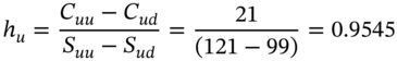
The outcomes at the D-node and U-node are equal since the hedge is designed so that ![]() . At the U-node, the new hedge ratio
. At the U-node, the new hedge ratio ![]() . As we have 1,000 written options then we need to hold 954.5 stocks. Hence we buy an additional (954.5 – 750) stocks @
. As we have 1,000 written options then we need to hold 954.5 stocks. Hence we buy an additional (954.5 – 750) stocks @ ![]() using borrowed funds at an interest cost
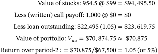
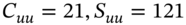
using borrowed funds at an interest cost ![]() . The outcomes at the UU-node and UD-node are:
. The outcomes at the UU-node and UD-node are:
- UU-node:
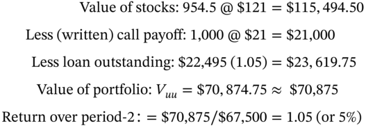
- UD-node:
To reach the D-node from t = 0 we move from holding 750 stocks ![]() to zero stocks, since at node-D,
to zero stocks, since at node-D, ![]() . Selling 750 stocks at
. Selling 750 stocks at ![]() results in a cash inflow of $67,000. The 1,000 written calls sold at
results in a cash inflow of $67,000. The 1,000 written calls sold at ![]() are worth zero, at node-DD. (Notionally, we could buy back 1,000 calls at a cost of
are worth zero, at node-DD. (Notionally, we could buy back 1,000 calls at a cost of ![]() .) The cash inflow of $67,000 is the same as
.) The cash inflow of $67,000 is the same as ![]() calculated above.
calculated above.
Explaining the move from node-D, to either node-DD or node-UD is trivial. We have ![]() stocks which are worth zero at nodes UD and DD and the calls are also worth zero
stocks which are worth zero at nodes UD and DD and the calls are also worth zero ![]() .
.
Changing the Number of Calls in the Hedge
What would the hedge look like at node-U if we decided to change the number of calls (rather than the number of stocks) in order to maintain the delta hedge? At node-U the hedge ratio is ![]() and hence a hedged portfolio also consists of:
and hence a hedged portfolio also consists of:
Hold the ‘original’ 750 stocks and write 785.7 calls (= 750 / 0.9545)
At the outset we sold 1,000 calls and at node-U the delta hedge requires 785.7 written calls, hence we must buy back 214.3 calls:
At node-U buy back 214.3 calls @ $15 = $3,214 (= borrowed funds)
We can show that delta hedging by changing the number of calls produces the same outcomes as our above analysis (i.e. with a fixed 1,000 written calls). For example, the outcome at the UU-node of our ‘new’ hedge is:
- UU-node:
This is exactly the same payoff as when we hedged at node-U using a fixed 1,000 written calls and delta hedging with 954.5 stocks. In fact the latter is a more realistic outcome as options traders in banks tend to be net sellers of calls to their retail and corporate customers and they dynamically delta-hedge this position by changing their stock holdings, day-by-day until the maturity date of the option (or until they close out their options position prior to maturity).
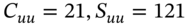
Making arbitrage profits from a mispriced call with two periods to maturity is similar to that for the one-period case, except the ‘arbitrage profit’ may accrue in either or both of the two periods depending on when the mispricing is corrected. Clearly if the mispricing is not corrected in the first period, the ‘delta-hedged’ calls and stocks earn the risk-free rate. But in the second period the mispricing must be corrected, since the option reaches maturity. Then a return in excess of the risk-free rate is earned between ![]() and
and ![]() – hence over the two periods, the arbitrageur earns more than the risk-free rate.
– hence over the two periods, the arbitrageur earns more than the risk-free rate.
For example, suppose a call is initially overpriced. At ![]() you sell 1 call and buy h stocks. If the mispricing is not corrected in period-1 then you earn the risk-free rate. But if the mispricing is corrected, the call becomes correctly priced at the end of the first period, and you earn more than the risk-free rate over period-1 – in this case you earn the risk-free rate in period-2 since the mispricing has already been corrected.
you sell 1 call and buy h stocks. If the mispricing is not corrected in period-1 then you earn the risk-free rate. But if the mispricing is corrected, the call becomes correctly priced at the end of the first period, and you earn more than the risk-free rate over period-1 – in this case you earn the risk-free rate in period-2 since the mispricing has already been corrected.
EXERCISES
Question 1
How are the size of the ‘up’ moves (U) and ‘down’ moves (D) determined in the BOPM and how is the stock price volatility represented in the tree for the BOPM?
Question 2
For a binomial tree with ![]() periods there are
periods there are ![]() possible paths to arrive at the final values for the stock price.
possible paths to arrive at the final values for the stock price.
- List these 8 different paths (to reach the stock prices at
 ).
). - How many distinct values for the stock price are there at
 ?
? - How many alternative ways (paths) are there to reach a node at
 which has (i) two up moves, or (ii) two down moves, (iii) 3 up moves, (iv) 3 down moves? List these alternative paths.
Question 3
In the BOPM, when delta hedging an option position, why does the hedge position have to change as you move through the lattice?
Question 4
In the BOPM, give an intuitive interpretation using risk neutral valuation, of the formula for the put premium on a stock, with two periods to expiration:
where ![]() ,
, ![]() and
and ![]() .
.
Question 5
How can you use ![]() held in a risk-free asset (e.g. a zero-coupon bond or bank deposit/loan) together with
held in a risk-free asset (e.g. a zero-coupon bond or bank deposit/loan) together with ![]() stocks with current price
stocks with current price ![]() , to replicate the payoff to a one-period (long) European put? What does this imply for the number of stocks to buy or sell to replicate the put payoff?
, to replicate the payoff to a one-period (long) European put? What does this imply for the number of stocks to buy or sell to replicate the put payoff?
Briefly explain what happens in your replication strategy if the stock price increases by $2 (over a short time horizon).
Question 6
Consider the two-period BOPM. The current stock price ![]() and the risk-free rate
and the risk-free rate ![]() per period (simple rate). Each period, the stock price can go either up by 10% or down by 10%. A European call option (on a non-dividend paying stock) with expiration at the end of two periods
per period (simple rate). Each period, the stock price can go either up by 10% or down by 10%. A European call option (on a non-dividend paying stock) with expiration at the end of two periods ![]() , has a strike price
, has a strike price ![]() .
.
- Draw the stock price tree (lattice).
- Show that the (no-arbitrage) price of the call is 12.47.
- Calculate the hedge ratio at
 .
. - Show how you can hedge 100 written calls at
 , and how the hedge portfolio earns the risk-free rate over the first period (i.e. along the path from node
  , either to node-D or node-U).
 - What would an investor do at
 if the call is overpriced at
  What is the outcome at
  (given that the stock price and the call premium are the same as in the lattice in parts (a) and (b))?
Question 7
Consider the two-period BOPM. The current stock price ![]() and the risk-free rate
and the risk-free rate ![]() per period (simple rate). Each period, the stock price can go either up by 10% or down by 10%. A European put option (on a non-dividend paying stock) expiring at the end of the second period has an exercise price of
per period (simple rate). Each period, the stock price can go either up by 10% or down by 10%. A European put option (on a non-dividend paying stock) expiring at the end of the second period has an exercise price of ![]() .
.
- Sketch the stock price tree (lattice).
- Calculate the fair (no-arbitrage) price of the put, P.
- Calculate the hedge ratio h, at time zero.
- Show how you can hedge 100 long puts at
 , and how the hedge-portfolio earns the risk-free rate over the first period (i.e. along the path from node
  , either to node-D or node-U).
 - What would an investor do at
 if the put is overpriced at
  What is the outcome at
  (if the stock price and the put premium are the same as in the lattice in parts (a) and (b))?
NOTES
- 1 The observant reader will have noted that we have not used this condition so far, yet we still obtained the correct (no-arbitrage) option prices using the binomial equation and the RNV approach. We get the correct option price because RNV does not allow any arbitrage profits to be made. What we have not done so far is to match the volatility of the stock price in the tree to its real world volatility
 , as measured by statisticians – this is because up to this point, for expositional purposes, we wanted to keep the numbers in the tree simple whole numbers, hence our choice of
  and
and  in our initial examples.
 - 2 To be more accurate (continuously compounded, log) stock returns are normally distributed but the distribution of the final stock price is actually lognormally distributed. This distinction need not concern us here.