CHAPTER 23
BOPM: Extensions
Aims
- To show how the BOPM is used to price American options – these are path-dependent options and subject to early exercise.
- To adapt the BOPM to price options on stocks that pay a continuous dividend, options on foreign exchange, and options on futures contracts.
- To use the BOPM to price options on stocks that pay dividends at discrete intervals.
- To demonstrate how the binomial approach can be speeded up using control variate techniques and trinomial trees.
- To show how stock price movements in the binomial tree are determined by the ‘real world’ volatility of stock returns.
23.1 AMERICAN OPTIONS
So far we have used the BOPM to price European options (which can only be exercised at maturity). American options can be exercised at any time, over the life of the option. The question arises as to when it is optimal to exercise an American option and how this affects the price of American options. The following results hold for American options:
- For a call option on a non-dividend paying stock, early exercise is never optimal.
- For a call option on a dividend paying stock, early exercise is sometimes optimal.
- For a put option on a stock (with or without dividends), early exercise is sometimes optimal.
As we shall see American options on stock indices, commodities, currencies and futures contracts can be priced using results for options on stocks that pay continuous dividends.
23.1.1 European Put
We price a two-period European put with ![]() using RNV. The tree for the stock price has
using RNV. The tree for the stock price has ![]() ,
, ![]() ,
, ![]() ,
, ![]() and the risk-neutral probability
and the risk-neutral probability ![]() . First we calculate the payoffs at maturity (Figure 23.1)
. First we calculate the payoffs at maturity (Figure 23.1) ![]() ,
, ![]() and
and ![]() . We then move backwards through the tree:
. We then move backwards through the tree:


FIGURE 23.1 European and American put
The (European) put premium is:

23.1.2 American Put
For an American put option the payoffs at maturity are the same as for the European put. But early exercise may be profitable at nodes ![]() and at
and at ![]() . To price the American put we see if the intrinsic value
. To price the American put we see if the intrinsic value ![]() (which is the cash received for early exercise) at any of the nodes is greater than the ‘recursive values’1 for the put,
(which is the cash received for early exercise) at any of the nodes is greater than the ‘recursive values’1 for the put, ![]() or
or ![]() (that is, the value of the put if you do not exercise it at that node). If
(that is, the value of the put if you do not exercise it at that node). If ![]() > ‘recursive value’ then early exercise is profitable and we replace the recursive value, ‘
> ‘recursive value’ then early exercise is profitable and we replace the recursive value, ‘![]() or
or ![]() ’ with the
’ with the ![]() at that node. Expressed mathematically the payoff to an American put at node-U is:
at that node. Expressed mathematically the payoff to an American put at node-U is:
At node-U, ![]() and
and ![]() so early exercise is not profitable and we retain
so early exercise is not profitable and we retain ![]() in the tree. At node-D,
in the tree. At node-D, ![]() and
and ![]() so early exercise is profitable and we replace
so early exercise is profitable and we replace ![]() in the tree with
in the tree with ![]() . The ‘recursive value’ at
. The ‘recursive value’ at ![]() now becomes:
now becomes:

Finally, we compare ![]() and
and ![]() , which indicates that early exercise is not profitable at
, which indicates that early exercise is not profitable at ![]() and hence the American put premium is
and hence the American put premium is ![]() . Notice that the American put is worth more than the equivalent European put (which has
. Notice that the American put is worth more than the equivalent European put (which has ![]() ) – the American put has extra ‘optionality’ as it allows for the possibility that early exercise may be profitable.
) – the American put has extra ‘optionality’ as it allows for the possibility that early exercise may be profitable.
This general principle of working backwards through the tree and seeing if early exercise is worthwhile applies when pricing all types of American options: on stock indices, currencies, futures contracts and commodities (e.g. corn, oil, gas etc.).
23.2 OPTIONS ON OTHER UNDERLYING ASSETS
It is convenient here to use the annual continuously compounded interest rate, denoted ![]() (decimal). One dollar today is worth
(decimal). One dollar today is worth ![]() after a small time interval
after a small time interval ![]()
![]() . The equation for the risk-neutral probability
. The equation for the risk-neutral probability ![]() when pricing an option on a stock which pays no dividends is:
when pricing an option on a stock which pays no dividends is:
23.2.1 Continuous Dividend Yield
If a stock has a continuous annual dividend yield ![]() (decimal), then the (total) return on the stock consists of the capital gain plus the dividend yield
(decimal), then the (total) return on the stock consists of the capital gain plus the dividend yield ![]() , where
, where ![]() is the growth (or proportionate change) in the stock price. In a risk-neutral world, the (total) return on a stock must equal the risk-free rate
is the growth (or proportionate change) in the stock price. In a risk-neutral world, the (total) return on a stock must equal the risk-free rate ![]() and hence, the expected growth in the stock price
and hence, the expected growth in the stock price![]() equals
equals ![]() and
and ![]() . In a risk-neutral world, the expected stock price at time
. In a risk-neutral world, the expected stock price at time ![]() is given by:
is given by:
Hence:
where ![]() .
.
When using the binomial recursion formula to price an option on a stock which pays continuous dividends at a (constant) rate ![]() , the only change required is that ‘
, the only change required is that ‘![]() ’ in the definition of
’ in the definition of ![]() is replaced by
is replaced by ![]() . The values
. The values ![]() and
and ![]() remain unchanged.
remain unchanged.
23.2.2 Options on Foreign Currency and Futures
To price options on a foreign currency, the equivalent to ![]() is the foreign risk-free rate
is the foreign risk-free rate ![]() . For options on a futures contract the underlying futures price grows at the rate
. For options on a futures contract the underlying futures price grows at the rate ![]() , hence the definitions for
, hence the definitions for ![]() become:
become:
- Option on foreign currency:

- Option on futures:

When setting up the tree, ![]() and
and ![]() remain unchanged and
remain unchanged and ![]() is the real world historical volatility of the underlying asset (i.e. volatility of the stock return, volatility of the return
is the real world historical volatility of the underlying asset (i.e. volatility of the stock return, volatility of the return ![]() on the exchange rate or the volatility of the return
on the exchange rate or the volatility of the return ![]() of the futures price, depending on the types of option being considered). Hence, the binomial tree for the underlying asset is constructed in the usual way. Hence, the only difference in the BOPM is the definition of ‘
of the futures price, depending on the types of option being considered). Hence, the binomial tree for the underlying asset is constructed in the usual way. Hence, the only difference in the BOPM is the definition of ‘![]() ’ (and hence
’ (and hence ![]() in Equation (23.4)).
in Equation (23.4)).
The maturity of the option ![]() is divided into
is divided into ![]() or more time steps, with each step
or more time steps, with each step ![]() – this gives a reasonably accurate value for the option's price. For a European option on a stock we only require the payoffs at maturity
– this gives a reasonably accurate value for the option's price. For a European option on a stock we only require the payoffs at maturity ![]() to price the option. For
to price the option. For ![]() time steps there are
time steps there are ![]() terminal stock prices – which is manageable. But for
terminal stock prices – which is manageable. But for ![]() there are
there are ![]() or about a billion alternative stock price paths (e.g. even for
or about a billion alternative stock price paths (e.g. even for ![]() there are 8 possible paths). Since many exotic options are path dependent, the BOPM with
there are 8 possible paths). Since many exotic options are path dependent, the BOPM with ![]() takes considerable computing power and it may take quite a while for the computer to ‘grind out’ a value for the option price. Hence various methods to speed up the calculations are used, such as trinomial trees and control variate techniques.
takes considerable computing power and it may take quite a while for the computer to ‘grind out’ a value for the option price. Hence various methods to speed up the calculations are used, such as trinomial trees and control variate techniques.
23.2.3 Control Variate Techniques
Control variate techniques can be used in the BOPM framework to obtain more accurate values for option premia (for any fixed number of nodes, in the tree). To illustrate this approach suppose we wish to price an American option – which is path dependent. If we value the American option using the standard BOPM with ![]() , this should give a good estimate of its true price. Assume this ‘true BOPM price’ is
, this should give a good estimate of its true price. Assume this ‘true BOPM price’ is ![]() – but computational time will be considerable.
– but computational time will be considerable.
To save on computational time, suppose we decide to price an American option using only ![]() steps in the BOPM and this gives
steps in the BOPM and this gives ![]() . In order to get closer to the true price
. In order to get closer to the true price ![]() , the control variate technique adjusts
, the control variate technique adjusts ![]() in the following way. First, we use the standard BOPM with
in the following way. First, we use the standard BOPM with ![]() to calculate the price of a European option
to calculate the price of a European option ![]() (on the same underlying, with the same strike and time to maturity). Both the American and European binomial prices with n = 5 are subject to error. However, we know the ‘exact’ Black–Scholes price for a European option
(on the same underlying, with the same strike and time to maturity). Both the American and European binomial prices with n = 5 are subject to error. However, we know the ‘exact’ Black–Scholes price for a European option![]() (say). Using the control variate technique, the price of the American option
(say). Using the control variate technique, the price of the American option ![]() is:
is:
The control variate technique adjusts the American binomial price ![]() (obtained using
(obtained using ![]() ), by the error in the BOPM estimate when pricing the (equivalent) European option,
), by the error in the BOPM estimate when pricing the (equivalent) European option, ![]() . If the BOPM overpriced the European option by 0.2 (with
. If the BOPM overpriced the European option by 0.2 (with ![]() ) we assume it will overprice the American option by the same amount. The control variate price
) we assume it will overprice the American option by the same amount. The control variate price ![]() is much closer to the ‘true’ price of the American option (using n = 100),
is much closer to the ‘true’ price of the American option (using n = 100), ![]() than the ‘unadjusted’ binomial estimate
than the ‘unadjusted’ binomial estimate ![]() with
with ![]() , and the control variate approach takes much less computing time.
, and the control variate approach takes much less computing time.
23.3 OPTIONS ON FUTURES CONTRACTS
Below, we show that RNV and backward recursion using the BOPM equation produces the same price for an option on a futures contract, as the ‘full no-arbitrage’ approach. A one-period call option on a futures contract delivers a long position in a futures contract. If the futures price at expiry of the option contract is ![]() and the strike is
and the strike is ![]() then a long call option at maturity can be cash settled for:
then a long call option at maturity can be cash settled for:
Suppose the risk-free rate ![]() (per period, continuously compounded),
(per period, continuously compounded), ![]() ,
, ![]() and
and ![]() , so
, so ![]() and
and ![]() . The payoffs for a one-period (
. The payoffs for a one-period (![]() ) call option on a futures contract with strike price
) call option on a futures contract with strike price ![]() are:
are:
We noted above that an option on a futures contract can be priced under RNV using:
which gives:
We now show that we obtain the same call premium using no-arbitrage and delta hedging. Suppose you are long one call at ![]() with (an unknown) call premium
with (an unknown) call premium ![]() . To create a risk-free portfolio you would short futures contracts, since if
. To create a risk-free portfolio you would short futures contracts, since if ![]() increases you would lose on the short futures but gain on the long call. If you short
increases you would lose on the short futures but gain on the long call. If you short![]() -futures for each long call then the payoffs at
-futures for each long call then the payoffs at ![]() are:
are:
To delta hedge we choose ![]() so these payoffs are equal, which implies:
so these payoffs are equal, which implies:

The cost of setting up the hedge portfolio at ![]() is simply the cost of the long call
is simply the cost of the long call ![]() , since it cost nothing to enter the futures contact. (We ignore margin payments.) Our portfolio of one long call and
, since it cost nothing to enter the futures contact. (We ignore margin payments.) Our portfolio of one long call and ![]() short futures is risk-free and must therefore earn the risk-free rate
short futures is risk-free and must therefore earn the risk-free rate ![]() (continuously compounded), otherwise arbitrage profits can be made. The cost of setting up the hedge portfolio at t = 0 is simply the cost of the call
(continuously compounded), otherwise arbitrage profits can be made. The cost of setting up the hedge portfolio at t = 0 is simply the cost of the call ![]() , financed using borrowed funds. At
, financed using borrowed funds. At ![]() the bank loan outstanding is
the bank loan outstanding is ![]() and for no arbitrage profits this must equal the known payoff on the hedge position
and for no arbitrage profits this must equal the known payoff on the hedge position ![]() (or
(or ![]() ):
):

We can obtain the solution for ![]() algebraically by substituting for
algebraically by substituting for ![]() from Equation (23.8) in (23.9), using
from Equation (23.8) in (23.9), using ![]() and
and ![]() and rearranging to give:
and rearranging to give:
Hence the ‘full no-arbitrage’ approach produces the same equation for the call premium as directly invoking RNV via (23.6b). Extending the above approach to the ![]() -period case, for European call or put futures options, is straightforward. We simply work backwards through the tree from
-period case, for European call or put futures options, is straightforward. We simply work backwards through the tree from ![]() to
to ![]() using
using ![]() .
.
23.3.1 American Futures Option
What about pricing an American futures option where we have the possibility of early exercise? To keep things simple, suppose we hold a two-period American call option on a futures contract. Early exercise at node-U is worthwhile if the intrinsic value ![]() , where the recursive formula gives
, where the recursive formula gives ![]() . If this is the case, we replace
. If this is the case, we replace ![]() in the tree by
in the tree by ![]() . This calculation is repeated for node-D (and at
. This calculation is repeated for node-D (and at ![]() ) – that is comparing
) – that is comparing ![]() , and
, and ![]() and then
and then ![]() and
and ![]() – and taking the maximum value in each case.
– and taking the maximum value in each case.
23.3.2 Numerical Example
Suppose an American call futures option has a time to maturity ![]() year, strike price
year, strike price ![]() and the current futures price is
and the current futures price is ![]() , with the volatility of the futures (return)
, with the volatility of the futures (return) ![]() p.a. We divide the time period
p.a. We divide the time period ![]() into
into ![]() periods so each step in the tree is
periods so each step in the tree is ![]() (which represents 1 month). We set
(which represents 1 month). We set ![]() and
and ![]() .
.
For a futures option ![]() so
so ![]() (and hence the option price is independent of the risk-free rate). The intrinsic value of the option at each node is
(and hence the option price is independent of the risk-free rate). The intrinsic value of the option at each node is ![]() . Let each node be denoted
. Let each node be denoted ![]() where
where ![]() and
and ![]() .
.
In Figure 23.2 the upper cells show the stock price and the lower cells the option value (price). At ![]() , the option is exercised at the two upper nodes, only. For
, the option is exercised at the two upper nodes, only. For ![]() and (2,2), the intrinsic value of the option exceeds its binomial recursive value – hence here the option is assumed to be exercised and the lower cells at these nodes show the option's intrinsic value
and (2,2), the intrinsic value of the option exceeds its binomial recursive value – hence here the option is assumed to be exercised and the lower cells at these nodes show the option's intrinsic value ![]() , rather than its binomial recursive value. The
, rather than its binomial recursive value. The ![]() s at these nodes are then used in calculating the next recursive values as we move backwards through the tree and the American call premium is 6.387. (As we increase the number of nodes in the tree, so that
s at these nodes are then used in calculating the next recursive values as we move backwards through the tree and the American call premium is 6.387. (As we increase the number of nodes in the tree, so that ![]() , we obtain a more accurate estimate of the call premium.)
, we obtain a more accurate estimate of the call premium.)
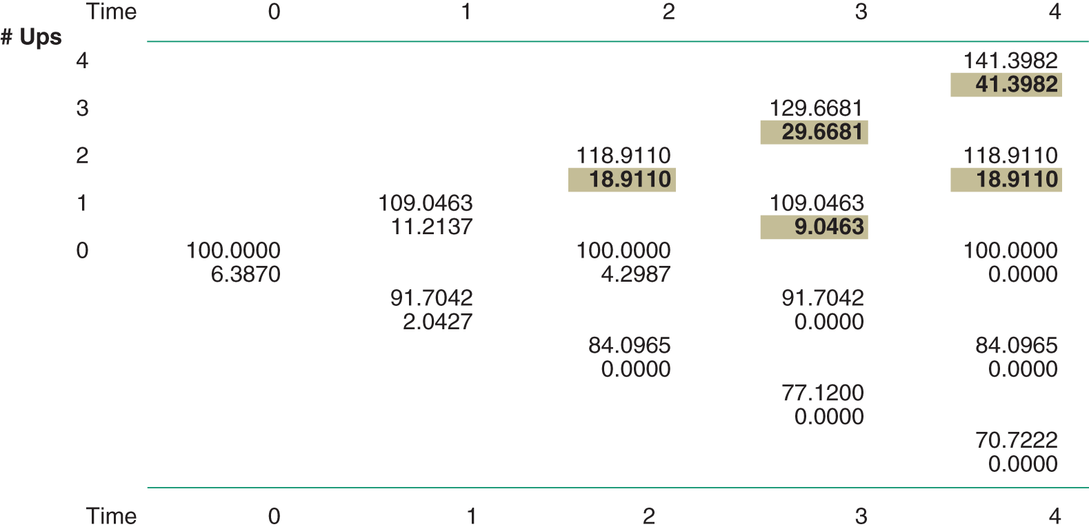
FIGURE 23.2 Binomial tree for American call on index futures
Note: Shaded areas indicate intrinsic value, used in the calculations.
For American options on stocks paying continuous dividends at a rate ![]() and options on FX, the procedure is the same as above. The tree is constructed using
and options on FX, the procedure is the same as above. The tree is constructed using ![]() and
and ![]() where
where ![]() is the real world (estimated annual) standard deviation of the stock return or FX return. Also
is the real world (estimated annual) standard deviation of the stock return or FX return. Also ![]() for the option on the stock and
for the option on the stock and ![]() for the FX-option (where
for the FX-option (where ![]() and
and ![]() ).
).
The BOPM can also be used to price options where the underlying asset is a stochastic interest rate (e.g. options on T-bonds, on T-bond futures or options on interest rates, known as caps and floors) but this requires a tree where interest rates are allowed to vary at each node. This is dealt with in Chapter 41.
23.4 OPTIONS ON DIVIDEND-PAYING STOCKS
23.4.1 Dividends and the BOPM
We have already seen that for a stock (or stock index) that pays a constant continuous dividend yield ![]() , we simply use
, we simply use ![]() as the risk-neutral probability and proceed in the usual fashion to price European or American options on the dividend paying stock (index). In practice, the continuously compounded dividend rate
as the risk-neutral probability and proceed in the usual fashion to price European or American options on the dividend paying stock (index). In practice, the continuously compounded dividend rate ![]() has to be estimated and clearly while the assumption of a constant dividend rate is not unreasonable for a stock index (which contains many stocks), it is not plausible for individual stocks, where dividend payments tend to be bunched in certain months of the year. The BOPM gets a little tricky when dividends are discrete.
has to be estimated and clearly while the assumption of a constant dividend rate is not unreasonable for a stock index (which contains many stocks), it is not plausible for individual stocks, where dividend payments tend to be bunched in certain months of the year. The BOPM gets a little tricky when dividends are discrete.
23.4.2 Single Known Dividend Yield
Assume the option matures in 30 days, ![]() ,
, ![]() so that
so that ![]() . We now apply the BOPM to a European call option where the underlying stock (index) pays a single dividend at time
. We now apply the BOPM to a European call option where the underlying stock (index) pays a single dividend at time ![]() . If the time
. If the time ![]() is prior to the stock going ex-dividend, the nodes on the tree correspond to stock prices:
is prior to the stock going ex-dividend, the nodes on the tree correspond to stock prices:
If time ![]() is after the stock goes ex-dividend the nodes would have values
is after the stock goes ex-dividend the nodes would have values
where ![]() is the known single dividend yield. For example, given a single dividend payment prior to the 2nd node, the binomial tree is shown in Figure 23.3. If there are several known dividend yields
is the known single dividend yield. For example, given a single dividend payment prior to the 2nd node, the binomial tree is shown in Figure 23.3. If there are several known dividend yields ![]() over the life of the option, then the nodes after the ex-dividend dates would be
over the life of the option, then the nodes after the ex-dividend dates would be ![]() .
.

FIGURE 23.3 Single dividend, known dividend yield
23.4.3 Known Dollar Dividend
First note that when a dividend is paid, the stock price falls by the amount of the dividend payment D. (We ignore any tax issues here.)2 If we let ![]() then unfortunately with discrete dividends, the binomial tree for
then unfortunately with discrete dividends, the binomial tree for ![]() does not recombine and there are a very large number of nodes to evaluate. To avoid this problem and obtain a recombining tree we proceed as follows. We let
does not recombine and there are a very large number of nodes to evaluate. To avoid this problem and obtain a recombining tree we proceed as follows. We let ![]() and
and ![]() apply to the stock price minus the present value of all known future dividends (over the life of the option), which we denote
apply to the stock price minus the present value of all known future dividends (over the life of the option), which we denote ![]() . Suppose a single ex-dividend date is at τ and the dividend paid is
. Suppose a single ex-dividend date is at τ and the dividend paid is ![]() . Then the values for
. Then the values for ![]() at times
at times ![]() are:
are:

The tree for ![]() is constructed using
is constructed using ![]() ,
, ![]() where
where ![]() .3 This gives us a recombining tree for
.3 This gives us a recombining tree for ![]() . To obtain a ‘new’ tree, we now add back the PV of future dividends, at each node. Suppose we have calculated
. To obtain a ‘new’ tree, we now add back the PV of future dividends, at each node. Suppose we have calculated ![]() at
at ![]() . Then a ‘new’ tree for
. Then a ‘new’ tree for ![]() at times
at times ![]() is:
is:

The option is then priced off this ‘new’ tree ![]() using
using ![]() as the risk-neutral probability.4
as the risk-neutral probability.4
For example, suppose ![]() , there is one dividend of $10 with an ex-dividend date at the end the second month (0.1667 years), then
, there is one dividend of $10 with an ex-dividend date at the end the second month (0.1667 years), then ![]() . If
. If ![]() then
then ![]() . We calculate the tree for
. We calculate the tree for ![]() using the above equations and then work backwards through the tree (from the maturity date of the option) to give the European call (or put) premium.
using the above equations and then work backwards through the tree (from the maturity date of the option) to give the European call (or put) premium.
To value an American call with strike ![]() on a dividend paying stock we would calculate the intrinsic value at each node and the early exercise decision is based on
on a dividend paying stock we would calculate the intrinsic value at each node and the early exercise decision is based on ![]() (not
(not ![]() ). For example, if the stock has just gone ex-dividend and at the next ‘upper node’
). For example, if the stock has just gone ex-dividend and at the next ‘upper node’ ![]() and the dividend at τ is
and the dividend at τ is ![]() then
then ![]() (since the present value of the dividend at τ is the dividend itself of $3). For an instant,
(since the present value of the dividend at τ is the dividend itself of $3). For an instant, ![]() and then ‘immediately’ it falls to $110 as it goes ex-dividend. But just before the stock goes ex-dividend the call has an intrinsic value of
and then ‘immediately’ it falls to $110 as it goes ex-dividend. But just before the stock goes ex-dividend the call has an intrinsic value of ![]() . If
. If ![]() at this node and this is greater than the recursive value
at this node and this is greater than the recursive value ![]() in the tree, then we replace
in the tree, then we replace ![]() with
with ![]() . We proceed in this way at each node, to see if the intrinsic value exceeds the recursive value. So, apart from the construction of the stock price tree, an American option on a stock which pays discrete dividends is priced in the usual way.
. We proceed in this way at each node, to see if the intrinsic value exceeds the recursive value. So, apart from the construction of the stock price tree, an American option on a stock which pays discrete dividends is priced in the usual way.
23.5 SUMMARY
- For options on a stock paying dividends at the continuous rate
 (decimal), the stock price tree is constructed using
  and
and  but the risk-neutral probability is now
 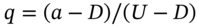 where
where  . The option is then priced in the usual way by backward recursion (under RNV).
 - For options on a foreign currency,
 the foreign interest rate and hence
  (where
  ),
),  and
and  (proportionate change) in the spot-FX rate.
 - For options on a futures contract,
 hence
hence  and
and  . In the tree
  is replaced by
  the forward rate, and
  is the volatility of
  .
. - American, European and many path-dependent ‘exotic options’ can be priced using the BOPM under RNV – so the method is very flexible.
- American options are valued using backward recursion but at each node we test to see if early exercise is profitable by comparing the intrinsic value
 (when exercised) with the binomial recursive value (no exercise), and we take the maximum of these two values. For example at node-U, the value of the put can be written
  , where
  is the BOPM recursive value.
 - To price an option on a stock that pays discrete dividends we construct a tree where we let
 and
and  apply to
  = ‘the stock price minus the present value of all known future dividends over the life of the option’. This allows the tree to recombine, which substantially improves computational efficiency. The option is then priced off a ‘new’ tree for
  where we add back the PV of future dividends, at each node. Expected payoffs are calculated using the (usual) risk-neutral probability,
 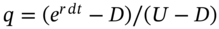 .
. - Computational time in the BOPM can be reduced by using control variate techniques or a trinomial tree (see Appendix 23).
APPENDIX 23: BOPM AND RISK-NEUTRAL VALUATION
As we see in Chapters 47 and 48, continuous time models of stock prices ![]() can be represented in terms of continuously compounded (‘log’) returns
can be represented in terms of continuously compounded (‘log’) returns ![]() or proportionate changes
or proportionate changes ![]() over a short period of time,
over a short period of time, ![]() . The ‘up’ and ‘down’ movements in the binomial tree for stock prices are an approximation to these continuous time processes and are designed to produce an outcome for the stock price
. The ‘up’ and ‘down’ movements in the binomial tree for stock prices are an approximation to these continuous time processes and are designed to produce an outcome for the stock price ![]() at
at ![]() , which is (approximately) lognormal. This requires movements of the stock price in the tree to replicate the ‘real world’ volatility of the stock price. In addition, when pricing options (on a non-dividend paying stock) using the BOPM under risk-neutral valuation (RNV), we must set the growth rate of the stock price equal to the risk-free rate.
, which is (approximately) lognormal. This requires movements of the stock price in the tree to replicate the ‘real world’ volatility of the stock price. In addition, when pricing options (on a non-dividend paying stock) using the BOPM under risk-neutral valuation (RNV), we must set the growth rate of the stock price equal to the risk-free rate.
In the BOPM we divide the time to maturity of the option ![]() (years) into
(years) into ![]() -periods of equal length,
-periods of equal length, ![]() . Over a small interval of time
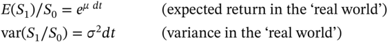
. Over a small interval of time ![]() , the expected return of the stock is measured as
, the expected return of the stock is measured as ![]() (where
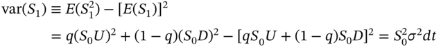
(where ![]() = continuously compounded annual growth rate, decimal). Over a small time interval, the variance of the stock return is
= continuously compounded annual growth rate, decimal). Over a small time interval, the variance of the stock return is ![]() (where
(where ![]() = annual standard deviation (decimal) of the continuously compounded stock return and is calculated from historical data). Hence:
= annual standard deviation (decimal) of the continuously compounded stock return and is calculated from historical data). Hence:
We price an option (on a non-dividend paying stock) using the BOPM under RNV. Therefore we calibrate ![]() ,
, ![]() and
and ![]() , so the stock price in the tree satisfies two conditions (over the time period
, so the stock price in the tree satisfies two conditions (over the time period ![]() ):
):
- Expected return equals the risk-free rate
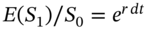 (RNV)
(RNV) - Variance of the stock price,
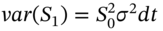 (‘real world’ volatility)
Hence, RNV and replicating the ‘real world’ volatility gives two equations and three unknowns (U, D, q):
From (23.A.1):
Multiplying (23.A.3) by ![]() and simplifying:
and simplifying:
Simplifying (23.A.2):
Substituting in (23.A.6) from (23.A.5) and (23.A.3):
We have three unknowns ![]() ,
, ![]() and
and ![]() and only two equations – the RNV equation (23.A.1) and the (simplified) volatility equation (23.A.7). We arbitrarily use our one ‘degree of freedom’ by setting
and only two equations – the RNV equation (23.A.1) and the (simplified) volatility equation (23.A.7). We arbitrarily use our one ‘degree of freedom’ by setting ![]() . Equation (23.A.1) or equivalently (23.A.3) gives directly:
. Equation (23.A.1) or equivalently (23.A.3) gives directly:
If higher order terms than ![]() are ignored, a solution to the volatility equation (23.A.7) (with
are ignored, a solution to the volatility equation (23.A.7) (with ![]() ) is:
) is:
In a risk-neutral world ![]() and
and ![]() are independent of the expected growth rate of the stock (i.e. the expected ‘real world’ stock return
are independent of the expected growth rate of the stock (i.e. the expected ‘real world’ stock return ![]() ), and therefore so is the option price. From (23.A.9) we have
), and therefore so is the option price. From (23.A.9) we have ![]() so U/D is determined by the ‘real world’ volatility of the stock return and hence so are the option premia.
so U/D is determined by the ‘real world’ volatility of the stock return and hence so are the option premia.
As we move from the ‘real world’ to our equations in a ‘risk-neutral’ world, the expected return on the stock changes from ![]() to
to ![]() (see 23.A.1) but the volatility of the stock return is the same as in the real world – this is a manifestation of Girsanov's theorem. It is easy to see that (23.A.9) satisfies the volatility equation (23.A.7) by substituting (the Taylor series approximations up to order
(see 23.A.1) but the volatility of the stock return is the same as in the real world – this is a manifestation of Girsanov's theorem. It is easy to see that (23.A.9) satisfies the volatility equation (23.A.7) by substituting (the Taylor series approximations up to order ![]() ):
):

in the left-hand side of (23.A.7) (and ignoring terms in ![]() or higher).
or higher).
The above analysis can be repeated for an option on an asset that pays a continuous yield (e.g. dividend yield) at a rate ![]() . The return on a stock equals the capital gain
. The return on a stock equals the capital gain ![]() plus the (continuously compounded, dividend) yield
plus the (continuously compounded, dividend) yield ![]() . In a risk-neutral world the asset (stock) return equals the risk-free rate
. In a risk-neutral world the asset (stock) return equals the risk-free rate ![]() and hence the expected value of the asset price
and hence the expected value of the asset price ![]() . Therefore, to price an option on an asset that pays a continuous yield, the only change in the above analysis is in (23.A.1) where we replace
. Therefore, to price an option on an asset that pays a continuous yield, the only change in the above analysis is in (23.A.1) where we replace ![]() with
with ![]() which results in
which results in ![]() in (23.A.8).
in (23.A.8).
Negative Risk-neutral Probabilities
Sometimes when ![]() is very small, the above formulas can give negative probabilities for
is very small, the above formulas can give negative probabilities for ![]() – which are meaningless. One ‘trick’ to avoid this problem is to assume the option is written on a futures contract with futures price
– which are meaningless. One ‘trick’ to avoid this problem is to assume the option is written on a futures contract with futures price ![]() (even though in reality it is not!), then
(even though in reality it is not!), then ![]() and we never get negative risk-neutral probabilities. The tree for
and we never get negative risk-neutral probabilities. The tree for ![]() is constructed at each node and the underlying cash market price at each node is obtained using
is constructed at each node and the underlying cash market price at each node is obtained using ![]() , where
, where ![]() = constant dividend yield (or the foreign interest rate for a foreign currency option).
= constant dividend yield (or the foreign interest rate for a foreign currency option).
Other Risk-neutral Probabilities
In the above derivation we found we had ‘one degree of freedom’ and imposed ![]() (Cox, Ross and Rubinstein 1979). This gives unique values for
(Cox, Ross and Rubinstein 1979). This gives unique values for ![]() ,
, ![]() and
and ![]() with which to construct the binomial tree, which is then used to price the option. But we could have used another ‘trick’ in the derivation of
with which to construct the binomial tree, which is then used to price the option. But we could have used another ‘trick’ in the derivation of ![]() ,
, ![]() and
and ![]() , which results in
, which results in ![]() being the same for options with different underlying assets, S (e.g. options on stocks that pay no dividends, on stocks that pay continuous dividends, options on FX-spot rates or commodities or futures contracts).
being the same for options with different underlying assets, S (e.g. options on stocks that pay no dividends, on stocks that pay continuous dividends, options on FX-spot rates or commodities or futures contracts).
This seems a little counter-intuitive but it is to do with how we ‘allocate’ our one degree of freedom. Given our two equations to determine the three ‘unknowns’ ![]() ,
, ![]() and
and ![]() we can arbitrarily set
we can arbitrarily set![]() . Then solving our two equations (23.A.3) and (23.A.7) for
. Then solving our two equations (23.A.3) and (23.A.7) for ![]() and
and ![]() we obtain (when terms of higher order than
we obtain (when terms of higher order than ![]() are ignored):
are ignored):
Clearly, using these values of ![]() and
and ![]() would give a different tree for the stock price than if we use the Cox, Ross and Rubinstein formulas but the value of the option premium from backward recursion using the BOPM under RNV is the same using either approach. The different values for
would give a different tree for the stock price than if we use the Cox, Ross and Rubinstein formulas but the value of the option premium from backward recursion using the BOPM under RNV is the same using either approach. The different values for ![]() in the two trees would exactly offset the different values for
in the two trees would exactly offset the different values for ![]() , and the price of the option using backward recursion turns out to be the same. (After all we can only have one ‘correct’ or ‘no-arbitrage’ price for the option.)
, and the price of the option using backward recursion turns out to be the same. (After all we can only have one ‘correct’ or ‘no-arbitrage’ price for the option.)
For a stock (index) paying a continuous dividend at a rate ![]() , we replace
, we replace ![]() by
by ![]() in Equations (23.A.10a) and (23.A.10b):
in Equations (23.A.10a) and (23.A.10b):
In addition, for currency options ![]() the foreign interest rate and for options on futures contracts
the foreign interest rate and for options on futures contracts ![]() , so
, so ![]() is omitted from the above equations. Hence, Equations (23.A.11a) and (23.A.11b) enable construction of a tree for the underlying asset and hence price options on dividend paying stocks, currencies and futures contracts when using
is omitted from the above equations. Hence, Equations (23.A.11a) and (23.A.11b) enable construction of a tree for the underlying asset and hence price options on dividend paying stocks, currencies and futures contracts when using ![]() .
.
Note that the size of ![]() and D (and the value of
and D (and the value of ![]() ) have all been derived assuming a risk-neutral world. So, when pricing options, the tree for the stock price does not represent actual movements in the stock price but it still correctly prices the option because of the equivalence of backward recursion using RNV and the ‘no-arbitrage’ approach.
) have all been derived assuming a risk-neutral world. So, when pricing options, the tree for the stock price does not represent actual movements in the stock price but it still correctly prices the option because of the equivalence of backward recursion using RNV and the ‘no-arbitrage’ approach.
Trinomial Tree
When pricing an option, the use of a trinomial tree rather than a binomial tree can reduce computational time. The tree is set up so that at each node there is an up, middle, and down step. For example, for a non-dividend paying stock, the tree mimics the ‘real world’ volatility and has the stock price growing at the risk-free rate if:

where ![]() ,
, ![]() ,
, ![]() are the risk-neutral probabilities for the down move, up move and for the ‘middle’ path. We then use backward recursion on the trinomial tree to calculate the option premium. For assets paying a continuous dividend yield at a rate
are the risk-neutral probabilities for the down move, up move and for the ‘middle’ path. We then use backward recursion on the trinomial tree to calculate the option premium. For assets paying a continuous dividend yield at a rate ![]() , we replace
, we replace ![]() by
by ![]() in the above equations. Also, for currency options
in the above equations. Also, for currency options ![]() the foreign interest rate and for options on futures
the foreign interest rate and for options on futures ![]() , so
, so ![]() is omitted from the above equations. The trinomial tree is equivalent to the explicit finite difference method, discussed in Chapter 48.
is omitted from the above equations. The trinomial tree is equivalent to the explicit finite difference method, discussed in Chapter 48.
EXERCISES
Question 1
Why is the BOPM (and other ‘tree methods’) often seen to be more flexible than closed-form solutions for the options price, such as the Black–Scholes formula for calls and puts?
Question 2
What are the drawbacks of using the BOPM to price options?
Question 3
You want to price an American put option (on a non-dividend paying stock) using the BOPM with ![]() steps. How does the control variate technique improve the accuracy of the price of the American put? Explain.
steps. How does the control variate technique improve the accuracy of the price of the American put? Explain.
Question 4
You hold a long (European) put option on a futures contract. The current futures price is ![]() and the futures price can move to either
and the futures price can move to either ![]() or
or ![]() . The futures option has a strike price
. The futures option has a strike price ![]() ,
, ![]() period to maturity and the risk-free rate
period to maturity and the risk-free rate ![]() p.a. (continuously compounded).
p.a. (continuously compounded).
- Create a risk-free portfolio consisting of one long put and futures contracts.
- Using the no-arbitrage condition, calculate the European put premium.
- Check that the value of your hedge portfolio is the same at the up and the down nodes.
- Check your answer in (b) by using the BOPM formula for the price of the put option.
Question 5
The index futures price is ![]() . An American put option on the futures index has
. An American put option on the futures index has ![]() ,
, ![]() p.a. (continuously compounded),
p.a. (continuously compounded), ![]() p.a.,
p.a., ![]() year (4 months).
year (4 months).
Use a tree with ![]() steps to calculate the ‘up’ and ‘down’ moves for the futures price and show that the price of the American put is
steps to calculate the ‘up’ and ‘down’ moves for the futures price and show that the price of the American put is ![]() .
.
Question 6
The spot FX-rate is ![]() ($/£, USD per GBP). An American put option on the USD has
($/£, USD per GBP). An American put option on the USD has ![]() (USD/GBP), the interest rate in the US is
(USD/GBP), the interest rate in the US is ![]() p.a. (continuously compounded), the volatility of the USD-GBP spot exchange rate
p.a. (continuously compounded), the volatility of the USD-GBP spot exchange rate ![]() p.a., the option has
p.a., the option has ![]() year to maturity and the interest rate in the UK is
year to maturity and the interest rate in the UK is ![]() p.a. (continuously compounded).
p.a. (continuously compounded).
Use a tree with ![]() steps to calculate the ‘up’ and ‘down’ moves for the spot FX-rate and show that the price of the American put is
steps to calculate the ‘up’ and ‘down’ moves for the spot FX-rate and show that the price of the American put is ![]() (USD/GBP).
(USD/GBP).
NOTES
- 1 The ‘recursive value’ is also referred to as the ‘continuation value’, since option values at each node of the lattice/tree depend on option values in future time periods.
- 2 This occurs because if the stock price were to fall by less than D (e.g.
 ) then you could buy the stock for S immediately prior to the ex-dividend date, capture the dividend D and immediately sell the stock for S – Z. Your
  (ignoring any problems due to discounting, when dividends are paid with a lag).
 - 3
 is slightly larger than
  , the volatility of
  . In practice the input for
  is usually an implied volatility.
 - 4 Note that (perhaps surprisingly) the formula for
 is for an option on a stock that does not pay dividends. This is because we have adjusted the values of
  in the tree to reflect dividend payments, so to use
  would be a form of ‘double counting’.
 - 5 Here we use the standard result,