
Chapter 13. Camera Specifications and Transformations
13.1. Introduction
In this chapter, we briefly discuss camera specifications, which you already encountered in Chapter 6. Recall that we specified a camera in WPF in code like that shown below:
1 <PerspectiveCamera
2 Position="57, 247, 41"
3 LookDirection="-0.2, 0, -0.9"
4 UpDirection="0, 1, 0"
5 NearPlaneDistance="0.02" FarPlaneDistance="1000"
6 FieldOfView="45"
7 />
From such a specification, we will create a sequence of transformations that will transform the world coordinates of a point on some model to so-called “camera coordinates,” and from there to image coordinates. We’ll do so by repeatedly using the Transformation Uniqueness principle.
Since an affine coordinate frame in three dimensions consists of four noncoplanar points, this says that if we know where we want to send each of four noncoplanar points, we know that there’s exactly one affine transformation that will do it for us. The corresponding theorem for the plane says that if we know where we want to send some three noncollinear points, then there’s a unique affine transformation that will do it.
We start with an example of this kind of transformation in the plane. Next we discuss basic perspective camera specifications and how we can convert such specifications to a set of affine transformations, plus one projective transformation. We briefly treat the case of “parallel” cameras, and discuss the details of that case and of skewed projections, in this chapter’s web materials.
13.2. A 2D Example
While Chapter 10 showed how to build transformations and compose them, it’s often easiest to use a higher-level construction to build transformations: Rather than saying how to create a transformation as a sequence of elementary transformations, we say what we want the transformation to accomplish. Using our linear algebra package (see Chapter 12), we can simply say that we want a linear map that takes certain points to certain others, and let the package find the unique solution to this problem.
Suppose we want to map the square –1 ≤ u, v ≤ 1 (which we’ll call the imaging rectangle in anticipation of a later use of such a transformation) to a display with square pixels, 1024 pixels wide, 768 pixels tall. The upper-left pixel is called (0, 0); the lower-left is (0, 767); and the lower-right is (1023, 767). We want to find a transformation T with the property that it sends the square –1 ≤ u, v ≤ 1 to a square region on the left-hand side of the display, one that fills as much of the display as possible. To do so, we need coordinates on the plane of the display. Because pixel coordinates refer to the upper-left corner of each pixel, as shown in Figure 13.1, that is, the center of pixel (0, 0) is at (0.5, 0.5), the display coordinates range from (0, 0) to (1024, 768).
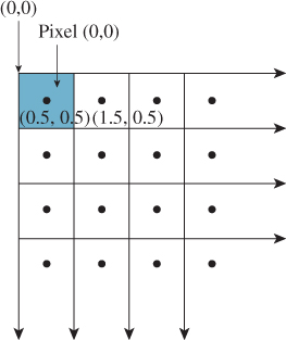
Figure 13.1: The center of the upper-left pixel has coordinates (0. 5, 0. 5); the pixel is called pixel (0,0). In other words, it is named by its upper-left corner.
This means that we want the point (–1, –1) (the lower-left corner of the imaging rectangle) to be sent to (0, 768) (the lower-left corner of the display), and we want (–1, 1) (the upper-left corner) to be sent to (0, 0). To completely specify an affine transformation on a two-dimensional space, we need to know where three independent points are sent. We’ve already determined where two are sent. For our third point, we choose the lower-right corner: (1, –1) must go to (768, 768) (to keep the image square). The code that implements this is
1 Transform t =
2 Transform.PointsToPoints(
3 Point2(-1, -1), Point2(-1, 1), Point2(1, -1),
4 Point2(0, 768), Point2(0, 0), Point2(768, 768));
For a specification like this (specifying which points go to which points) we must be certain that the source points constitute a coordinate frame; in two dimensions, this means “noncollinear,” which is clearly the case here: Any three corners of a square are noncollinear.
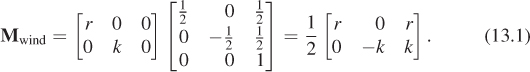
The obvious generalization of this to an arbitrary viewing window of r rows by k columns (without the constraint on squareness) is called the windowing transformation, with matrix Mwind. It can be generated by code like
1 Transform t =
2 Transform.PointsToPoints(
3 Point2(-1, -1), Point2(-1, 1), Point2(1, -1),
4 Point2(0, k), Point2(0, 0), Point2(r, k));
or, for those who prefer the matrix to be expressed directly, as
13.3. Perspective Camera Specification
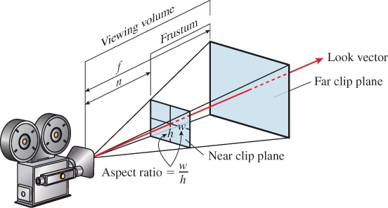
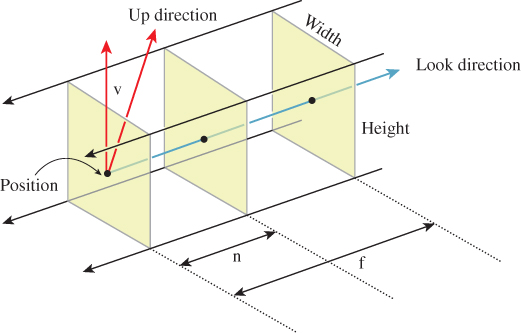
The WPF camera specification uses six parameters to specify a camera: position (a point), look direction and up direction (two vectors), near-plane distance and far-plane distance (two scalars), and field of view (an angle in degrees).
Figure 13.2 shows these. You can think of the camera being specified as a pinhole camera so that all rays entering the camera do so through a single point, specified as the position of the camera. You could also think of this as the center of the camera lens in a more conventional camera. In setting up a real-world photograph, we generally establish several things: the camera position, its orientation, and the field of view (often adjusted with a zoom control on the camera). For fancier cameras, we may also be able to adjust the focal distance (the distance to the points that are most in focus in the image), the depth of field (how far in front of and behind the focal distance things will be in focus), and even the tilt and offset of the camera lens relative to the camera body. The WPF specification, and that of most basic graphics systems, omits these latter aspects, since an ideal pinhole camera is in focus at all depths, and the pinhole is typically centered over the film or imaging sensor. We’ll return to these topics in Section 13.9.
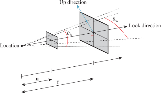
Returning to the WPF camera model, the look direction specifies in which direction the camera is pointed. If we trace a ray in the scene starting at the position and pointing in the look direction, we’ll hit some object. That object will appear in the exact center of the “picture” taken by our camera. The field-of-view angles describe how far from the look direction, in degrees, the camera sees. The basic WPF camera produces a square picture, so the field of view is the same in both the horizontal and vertical directions. In some other systems, you get to specify both a horizontal and vertical field of view (see Exercise 13.1). Others, including WPF, let you specify both the aspect ratio and the horizontal field of view, and compute the vertical field of view for you. In fact, in WPF you specify the aspect ratio indirectly. You specify the width and height of the viewport (a rectangle on the display used for exhibiting the image), and the aspect ratio is determined by the ratio of the width to the height. In the remainder of our presentation, we’ll specify the view in terms of both horizontal and vertical field of view, and we’ll discuss the relationship to aspect ratio afterward.
The only subtle point is the specification of the up direction, which orients the camera about the look direction, just as you can look out a window with your head tilted either left or right. If we imagine a vertical unit vector v painted on the back of the camera body, then this vector, together with the look direction, determines a plane. You might think that we should require the user to specify the vector v directly, but that’s rather difficult to do in general. Instead, we require the user to specify any nonzero vector in the plane (except the look direction), and from this we compute the vector v. Figure 13.3 shows this: Any of three different vectors can be used as the up direction, from which we can compute the vector v that is in the vertical plane of the camera and is perpendicular to the look direction. Often in practice the UpDirection is set to Vector3D(0,1,0), that is, the y-direction. As long as the camera does not look straight up or down, this is the most natural direction in which to hold it.1 If the camera does look straight up, then the computed vector v will be zero; if the camera looks nearly straight up, the computation of v from vup will involve division by a number that’s almost zero, and hence will be numerically unstable.
1. In CAD, the horizontal plane is often xy, with z used for the vertical direction; in that case, of course, the up vector would be Vector3D(0,0,1).
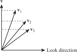
Figure 13.3: The vectors v1, v2, and v3 all lie in the plane of LookDirection and v, and any one of them can be used as the UpDirection and result in the same view.
At this point, the view specification tells where the camera is, in which direction it’s looking, and how the camera body is rotated around that view direction; the field of view determines how wide an area the camera “sees.” We’ve indirectly described a four-sided view volume with a rectangular cross section in space.
Two more parts of the specification remain: the near-plane and far-plane distances shown in Figure 13.4. The near and far planes cut out a frustum of the view cone. Objects within this frustum will be displayed in our image, but objects outside will not (see Figure 13.5).
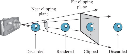
This can be a useful device: By setting the near-plane distance to be almost the distance to the subject, we guarantee that objects between us and the subject do not interfere with the picture. We also avoid ever considering objects that are behind the camera, which can be a huge time-saver. And by setting the far-plane distance so that it is not too large, we can similarly save lots of time, by never considering all the objects in the world that are potentially within our view but would hardly affect it at all, such as a person standing 30 miles away.
It is not only the utility of being able to set the near- and far-plane distances that motivates their use, as you’ll see presently; they also allow a rasterizing renderer to avoid certain floating-point-comparison problems that generate errors in images.
Clipping planes have often been used in games to help reduce rendering time by removing distant objects, but sometimes as you move forward in a game, a distant object will “pop” into view, which can be distracting. The general solution to this problem was to render objects in the distance as being obscured by fog so that they appeared gradually as you approached them. In more modern games, we have better rendering systems, and many objects are represented with multiple different levels of detail (see Section 25.4) so that when they are distant, they can be rendered with fewer polygons, making the use of fog less common than it once was.
13.4. Building Transformations from a View Specification
We’ll now convert from a view specification to some specific geometry. From a specification, we’ll build (a) an orthonormal coordinate system based at the camera position, and (b) several points on the view cone, as shown in Figure 13.6. We’ll use these in building the transformations we need. Having a coordinate frame based at the camera is very convenient, since we’ll later be transforming the camera to the origin and aligning its coordinate frame with the standard xyz-coordinate system at the origin.
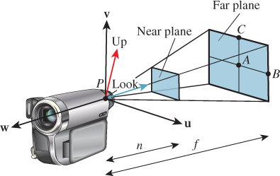
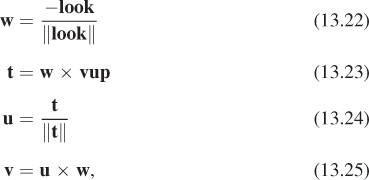
In writing the equations, we’ll use vup and look to indicate the up vector and look direction, respectively; these shorter names make the equations more comprehensible. The point P is just a shorter name for the camera’s Position.
We’ll build the orthonormal basis, u, v, w, in reverse order. First, w is a unit vector pointing opposite the look direction, so
To construct v, we first project vup onto the plane perpendicular to w, and hence perpendicular to the look direction as well, and then adjust its length:
Finally, to create a right-handed coordinate system, we let
Some camera software (like Direct3D, but not OpenGL) starts by letting w = S(look), without negation.
(a) Show that this makes no difference in the computation of v.
(b) Show that in this case, if we want u, v to retain the same orientation on the view plane (i.e., u pointing right, v pointing up), then the computation of u becomes u = w × v.
(c) Is the resultant uvw-coordinate system right- or left-handed?
Now we’ll compute the four points P, A, B, and C. The only subtlety concerns determining the length of edges AB and AC. The edge AB subtends half the horizontal field of view at P, and is at distance f from P, so
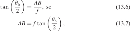
where θh denotes the horizontal field of view angle, converted to radians,
and similar expressions determine θv, the vertical field of view, and the length of AC:
Notice that the near-plane distance n has not entered into our computations yet.
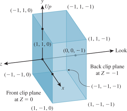
We now use the four points P, A, B, and C to transform the view frustum to the standard view frustum shown in Figure 13.7, and known as the standard perspective view volume.
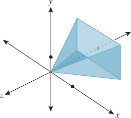
Figure 13.7: The standard perspective view volume is the pyramid that ranges from -1 to 1 in x and y, and from 0 to -1 in z. The scale in z is exaggerated.
All we need to do is say where the four points should be sent. We want to send P to the origin, A to the midpoint of the back face, which is (0, 0, –1), B to the mid-right edge of the back face, which is (1, 0, –1), and C to the mid-top edge, which is (0, 1, –1). The matrix that performs this transformation is denoted Mper (for “perspective”), so we’ll call the associated transformation Tper. The code that creates our transformation is
1 Transform3 Tper =
2 Transform3.PointsToPoints(
3 P, A, B, C,
4 Point3(0, 0, 0), Point3(0, 0, -1)), Point3(1, 0, -1), Point3(0, 1, -1));
Under this transformation, points of the far plane are transformed to the z = –1 plane. Since distances along the ray from P to A must transform linearly, points of the near plane are transformed to the plane z = –n/f. We’re nearly done at this point: We’ve transformed the view volume to a standard view volume, and from this point onward, almost everything we’ll do is independent of the camera parameters, the exception being that the ratio –n/f will enter into some of our computations.
This may appear too simple to you. Indeed, in an earlier edition of this book, the development of the transformation took several pages. But it’s an example of the power of proving one good theorem and writing the associated code.
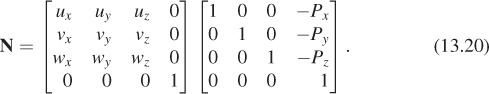
The transformation can also be realized step-by-step. We can take the camera’s view volume and apply a sequence of transformations to it: translate it so that P moves to the origin; rotate it several times around various coordinate axes so that the uvw-axes align with the xyz-axes; scale in z so that the far plane ends up at z = –1 instead of z = –f; and scale in x and y to make the view frustum have a width and height of 2. Letting Px, Py, and Pz denote the world coordinates of P, and similarly for u, v, and w, the matrix for the transformation is then
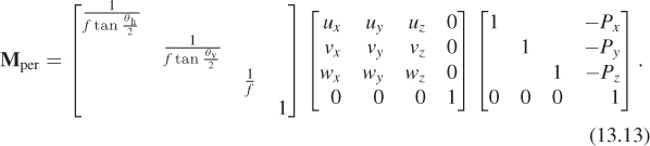
The rightmost matrix effects the translation; the middle one transforms u to e1, v to e2, and w to e3; the leftmost scales each axis appropriately.
We present these merely for your interest and strongly advocate using the PointsToPoints method instead, as it’s far less prone to errors in order of matrix multiplication, in copying of coordinates, etc.
At this point, it’s easy to project points in the standard perspective view volume onto the back plane, for instance, using the nonlinear transformation (x, y, z) ![]() (x/z, y/z, 1). This is more or less the process we followed when we rendered the cube in Chapter 3: Our uvw basis was already aligned with the xyz-axes, and our center of projection was chosen to be the center of our coordinate system, so all we had to do was the projection step.
(x/z, y/z, 1). This is more or less the process we followed when we rendered the cube in Chapter 3: Our uvw basis was already aligned with the xyz-axes, and our center of projection was chosen to be the center of our coordinate system, so all we had to do was the projection step.
Rather than take that approach, however, we’re going to apply two transformations—the first to “open up” our pyramidal view volume into a rectangular parallelepiped, and the second to project along the z-axis. There are two reasons for this.
• When we discuss “parallel” cameras and projections rather than the perspective cameras we’ve seen so far, the parallelepipedal volume will be a more natural target than the pyramidal one.
• When we project along the z-axis, it’s especially easy to determine which objects obscure which other objects, that is, visibility testing becomes trivial. This property is essential in the design of the so-called z-buffer algorithm at the heart of most graphics hardware.
Our standard parallel view volume (see Figure 13.8) is a parallelepiped that ranges from –1 to 1 in x and y, and from 0 to –1 in z. Its near clipping plane is z = 0; its far clipping plane is z = –1. (This differs from the parallel view volume used in either Direct3D or OpenGL, but only slightly.)
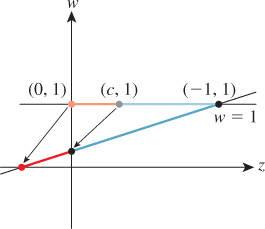
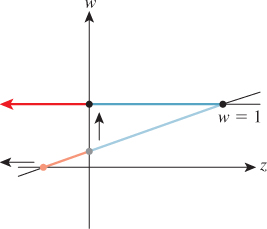
Now we’ll transform the portion of the standard perspective view volume between the transformed near and far planes (i.e., the portion between z = –n/f and z = –1) to the standard parallel view volume. The transformation we use will be a projective transformation in which all the rays passing from the view volume toward the origin are transformed into rays passing from the view volume toward the xy-plane in the positive-z direction (see Figure 13.9). (This is sometimes called an unhinging transformation, because the planes defining opposite sides of the view frustum meet along a “hinge line,” which this transformation “sends to infinity.”)
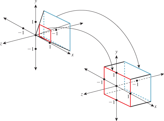
Applying this transformation has no impact on the final results of our rendering because the perspective projection (i.e., (x, y, z) ![]() (x/z, y/z, 1)) of a shape in the pre-transformed volume is the same as the parallel projection ((x, y, z)
(x/z, y/z, 1)) of a shape in the pre-transformed volume is the same as the parallel projection ((x, y, z) ![]() (x, y,1)) of the transformed shape in the post-transformed volume. This is easy to see if we look at a two-dimensional slice of the situation, just the yz-plane. Consider, for instance, the small square shown in Figure 13.10 that occupies the middle half of a perspective view of the scene. Occlusion (which points are obscured by others) is determined by the ordering of points along rays from the viewpoint into the scene so that the point B is obscured by the near edge of the square. After transformation, that ray from the viewpoint into the scene becomes a ray in the –z direction; once again, the point B′ is obscured by the front edge of the square. And once again, the transformed square ends up filling the middle half of the parallel view of the scene. The essential underlying fact is that light (the underlying agent of vision) travels in straight lines, and the transformation we’ll build converts straight lines to straight lines (and in particular, the projection rays from the perspective view to projection rays for the parallel view).
(x, y,1)) of the transformed shape in the post-transformed volume. This is easy to see if we look at a two-dimensional slice of the situation, just the yz-plane. Consider, for instance, the small square shown in Figure 13.10 that occupies the middle half of a perspective view of the scene. Occlusion (which points are obscured by others) is determined by the ordering of points along rays from the viewpoint into the scene so that the point B is obscured by the near edge of the square. After transformation, that ray from the viewpoint into the scene becomes a ray in the –z direction; once again, the point B′ is obscured by the front edge of the square. And once again, the transformed square ends up filling the middle half of the parallel view of the scene. The essential underlying fact is that light (the underlying agent of vision) travels in straight lines, and the transformation we’ll build converts straight lines to straight lines (and in particular, the projection rays from the perspective view to projection rays for the parallel view).
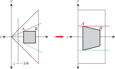
Figure 13.10: The standard perspective view volume at left (with a near clipping plane at z = –1/4) contains a small square, which is transformed into a parallelogram in the parallel view volume at right.
Recall from Section 11.1.1 that a projective transformation on R3 can be written as a linear transformation on R4 (the homogeneous-coordinate representation of points in 3-space), followed by the homogenizing transformation
Letting ![]() denote the z-coordinate of the front clipping plane after transformation to the standard perspective view volume (here at last the parameter n is being used!), we’ll simply write down the linear transformation from perspective to parallel, which we call Mpp:
denote the z-coordinate of the front clipping plane after transformation to the standard perspective view volume (here at last the parameter n is being used!), we’ll simply write down the linear transformation from perspective to parallel, which we call Mpp:
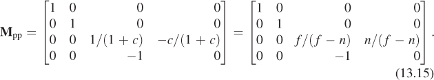
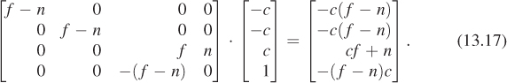
Because we’ll be homogenizing in a moment, we can multiply through by f – n and instead use the matrix
The derivation of this matrix is slightly messy and not particularly informative; we cover it in this chapter’s web materials. For now, all we need to do is verify that it does in fact transform the frustum between the near and far planes (z = c and z = –1, respectively) in the standard perspective view volume to the standard parallel view volume. We’ll do so by looking at corners.
Consider the upper-right front corner of the frustum. It’s at the location (–c, –c, c). (Recall that c = –n/f is negative, so –c is positive.) Under the transformation Mpp it becomes
Homogenizing, we get
the upper-right front corner of the standard perspective view volume, as promised, where the last step depends on ![]() .
.
Perform the corresponding computation for the lower-right rear vertex of the perspective view volume, and continue until you’re convinced that the transformation works as promised.
13.5. Camera Transformations and the Rasterizing Renderer Pipeline
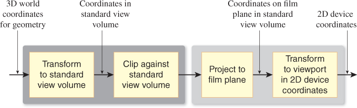
We described in Chapter 1 how graphics processing is typically done. First, geometric models, like the ones created in Chapter 6, are placed in a 3D scene by various geometric transformations. Then these models are “viewed” by a camera, which amounts to transforming their world-space coordinates into coordinates in the standard perspective view volume, and then transforming to the standard parallel view volume. Finally, they are projected to a 2D image, and this image is transformed to the viewport where we see a picture.
Along the way, the geometric representation of each model must be processed as shown in Figure 13.14. The 3D world coordinates of primitives (typically triangles) are “clipped” against a view volume; in other words, those outside the view volume are removed from consideration. A triangle that’s partly inside the view volume and partly outside may be truncated to a quadrilateral (and then typically subdivided into two new triangles). Alternatively, a system may determine that the truncation and retriangulation is more expensive than handling the small amount of work of generating pixel data that will never be shown; this depends on the architecture of the hardware doing the rasterization. The clipping operation is discussed in more detail in Chapters 15 and 36.
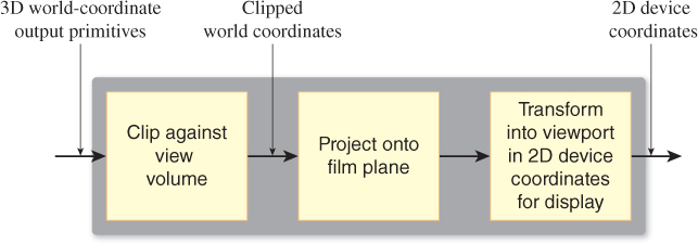
We’ll show how to implement this abstract rendering process in the context of camera transformations. Instead of clipping world coordinates against the camera’s view volume, we’ll transform the world coordinates to a standard view volume, where clipping is far simpler. In the standard view volume, we end up clipping against coordinate planes like z = –1, or against simple planes like x = z or y = –z. The projection to the film plane in the second step of the sequence is no longer a generic projection onto a plane in 3-space, but a projection onto a standard plane in the standard parallel view volume, which amounts to simply forgetting the z-coordinate. The revised sequence of operations is shown in Figure 13.15.
The dark gray section (the left half) of the sequence shown in Figure 13.15 can be further expanded for the perspective camera, as shown in Figure 13.16. In this case, we multiply by Mpp to transform from the standard perspective view volume to the standard parallel view volume, but before homogenizing, we clip out objects with z < 0. Why? Because an object with z < 0 and w < 0, after homogeneous division, will transform to one with z > 0 and w = 1. In practice, this means that objects behind the camera can reappear in front of it, which is not what we want.
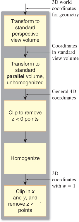
Following this first clipping phase, we can homogenize and clip against x and y and the far plane in z, all of which are simple because they involve clipping against planes parallel to coordinate planes.
To interpret the entire sequence of operations mathematically, we start with our world coordinates for triangle vertices and then do the following.
1. Multiply by MppMper, transforming points into the standard perspective view volume with Mper, and thence toward the standard parallel view volume (Mpp), stopping just short of homogenization.
2. Clip to remove points with z < 0. This, and step 4, actually requires knowledge of triangles rather than just the vertex data.
3. Apply the homogenizing transformation ![]() , at which point we can drop the w-coordinate.
, at which point we can drop the w-coordinate.
4. Clip against x = ±1, y = ±1, and z = –1.
5. Multiply by Mwind to transform the points to pixel coordinates.
This description omits two critical steps, which are the determination of the color at each vertex, and the interpolation of these colors across the triangles as we determine which pixels each triangle covers. The first of these was originally called lighting, as you learned in Chapter 2, but now the two together are often performed at each pixel by a small GPU program called a shader, and the whole process is therefore sometimes called “shading.” These are discussed in several chapters later in this book. For efficiency, however, it’s worth noting that lighting is an expensive process, so it’s worth delaying as late as possible so that you do the lighting computation for a vertex (or pixel) only if it makes a difference in the final image. The clipping stage is an ideal place to do this. You can avoid work for all the objects that are not visible in the final output. And for many basic lighting rules, it’s possible to do the lighting after transforming to the standard perspective view volume, or even after transforming to the standard parallel view volume, although not after homogenization.2 Because of this, it makes sense to do all the clipping in the pre-homogenized parallel view volume, then do the lighting, and finally homogenize, convert to pixel coordinates, and draw filled polygons with interpolated colors.
2. Many shading rules depend on dot products, and while linear transformations alter these in ways that are easy to undo, the homogenizing transformation’s effects are not easy to undo.
What about interpolation of colors over the interior of a triangle, given the color values at the corners? The answer is “It’s not as simple as it looks at first.” In particular, linearly interpolating in pixel coordinates will not work. To see this, look at the simpler problem shown in Figure 13.17: You’ve got a line segment PQ in the world, with a value—say, temperature—at each end, and the temperature is interpolated linearly along this line segment so that the midpoint is at a temperature exactly halfway between the endpoints, for instance. Suppose that line segment is transformed into the line segment P′Q′ in the viewport. If we take the midpoint ![]() and compute the point it transforms to, it will in general not be
and compute the point it transforms to, it will in general not be ![]() , so the temperature assigned to
, so the temperature assigned to ![]() should not be the average of the temperatures for P′ and Q′.
should not be the average of the temperatures for P′ and Q′.
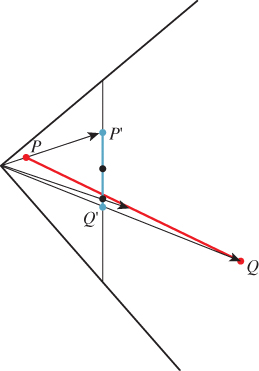
Figure 13.17: The projection of the midpoint of PQ is not the same as the midpoint of the segment P′Q′.
The only case where linear interpolation does work is when the endpoints P and Q are at the same depth in the scene (measured from the eye). The classic picture of train tracks converging to a point on the horizon provides a good instance of this. Although the crosspieces of the train track (“sleepers” in the United Kingdom, “ties” in the United States) are at constant spacing on the track itself, their spacing in the image is not constant: The distant ties appear very close together in the image. If we assign a number to each tie (1, 2, 3, ...), then the tie number varies linearly in world space, but nonlinearly in image space.
This suggests that interpolation in image space may be very messy, but the truth is that it’s also not as complicated as it looks at first. In Section 15.6.4.2 we will return to this topic and explain how to perform perspective-correct interpolation simply.
13.6. Perspective and z-values
Suppose we consider the perspective-to-parallel transformation Mpp for the case ![]() . (Recall that c = –n/f is the z-position of the near plane in the standard perspective view volume.) If we take a sequence of points equally spaced between c and –1 on the z-axis, and apply the transformation and homogenize, then we get a sequence of points between 0 and –1 in the parallel view volume, but they’re no longer equally spaced. Figure 13.18 shows the relationship of the new coordinates (z′) to the input coordinates (z) for several values of c. When c is near –1, the relationship is near linear; when c is near 0, the relationship is highly nonlinear. You can see how the output values all cluster near z′ = –1.
. (Recall that c = –n/f is the z-position of the near plane in the standard perspective view volume.) If we take a sequence of points equally spaced between c and –1 on the z-axis, and apply the transformation and homogenize, then we get a sequence of points between 0 and –1 in the parallel view volume, but they’re no longer equally spaced. Figure 13.18 shows the relationship of the new coordinates (z′) to the input coordinates (z) for several values of c. When c is near –1, the relationship is near linear; when c is near 0, the relationship is highly nonlinear. You can see how the output values all cluster near z′ = –1.
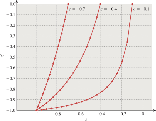
Figure 13.18: Points equispaced in depth in the perspective view volume transformed to unevenly spaced ones in the parallel view volume.
Now suppose that the z′-values are to be multiplied by N for some integer N and discretized to integer values between 0 and N – 1, as is common in many z-buffers, which use these discretized z′-values to determine which polygon is visible at a given pixel. If c is very small, then all the z′-values will be so near to 1 that they almost all discretize to N – 1, and the z-buffer will be unable to determine occlusion. In consequence, if you choose a near plane that’s too near the eye, or a far plane that’s too distant, then your z-buffer may not perform as expected. The near-plane distance is by far the more important: To avoid so-called z-fighting, you always want to push the near plane as far from the eye as possible while still seeing everything you need to see.
13.7. Camera Transformations and the Modeling Hierarchy
Recall that in Section 10.11 we made a hierarchy of transformations to represent the clock face of Chapter 2, and we said that a similar hierarchy could be created for a 3D model. For a 3D model, the product of all the matrices representing transformations from the world-coordinate system down to some primitive element (typically a triangle specified by its vertex coordinates) is called the composite modeling transformation matrix or CMTM.
This matrix, multiplied by the modeling coordinates of some vertex, produces the world coordinates of the corresponding point on the modeled object. (Remember that all coordinates need to be expressed homogeneously, to allow us to generate translations, so the CMTM is a 4 × 4 matrix.)
Explain why the last row of the CMTM, assuming that the transformations in the modeling hierarchy are all translations, rotations, and scaling transformations (i.e., they are all affine transformations), must be [0 0 0 1].
To transform world coordinates to the standard parallel view volume, we must multiply these coordinates by Mper and then Mpp, and then homogenize. The product
is called (in OpenGL) the modelview projection matrix or composite transformation matrix or CTM.
We can consider the uvw triple of vectors, determined by the camera specification, together with the camera location, as defining another coordinate system, eye coordinates. To transform a vertex from world to eye coordinates, we must multiply by the matrix
Confirm that N transforms P to the origin, transforms the vector u to [1 0 0 0]T, and similarly for v and w.
The product NCMTM is called the modelview matrix in OpenGL.
Suppose you’ve modeled a scene—two robots talking—and have placed a camera so as to view the scene. You want to show a friend the “larger context”—a more distant view of both robots and a geometric representation of the camera: a small pyramid whose vertex is at the eye. Fortunately, you happen to have a vertex-and-triangle-table representation of the standard perspective view volume, shortened by a factor of two in the y direction so that it’s twice as wide as it is tall. What transformation would you apply to this model to place it in the scene with its apex at the eye and its base parallel to the uv-plane, with its y-axis (the shorter one) aligned with v?
OpenGL defines another matrix—the projection matrix—that performs the transformation to the pre-homogenization standard parallel view volume. If we call this K, then the correspondence with the matrices we’ve defined is
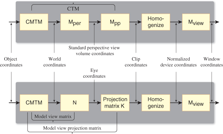
A comparison of the OpenGL sequence of transformations and ours is shown in Figure 13.19.
Let’s return to the two-robots-talking example. Assume that the first robot’s right hand is modeled as a unit cube (![]() ), with its
), with its ![]() face being attached to the wrist and its
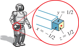
face being attached to the wrist and its ![]() face being the one that’s on top when the arms are held in front of the robot (see Figure 13.20), and that the CMTM for this cube is the matrix H. Now suppose that the hand is actually a camera whose eye position is at the center of the
face being the one that’s on top when the arms are held in front of the robot (see Figure 13.20), and that the CMTM for this cube is the matrix H. Now suppose that the hand is actually a camera whose eye position is at the center of the ![]() face (in modeling coordinates), shown as a red dot in the figure. The camera has a 90° field of view, both vertical and horizontal, a near-plane distance of 0. 5, and a far-plane distance of 10. Describe how to find Mper for this camera so that you can show what the first robot “sees” with its hand camera. Your answer should involve H.
face (in modeling coordinates), shown as a red dot in the figure. The camera has a 90° field of view, both vertical and horizontal, a near-plane distance of 0. 5, and a far-plane distance of 10. Describe how to find Mper for this camera so that you can show what the first robot “sees” with its hand camera. Your answer should involve H.
13.8. Orthographic Cameras
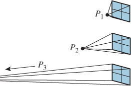
While perspective projections are familiar to us from ordinary photographs, many images are created using parallel projections or orthographic projections. In these projections, we project from the world to the film plane not using a collection of lines that all meet at the eyepoint, but instead using a collection of parallel lines. Imagine a perspective camera with a “film plane” at a fixed location in space, but whose eyepoint moves farther and farther from the film plane, resulting in the lines of projection becoming increasingly parallel (Figure 13.21); we can thus think of a parallel projection as a kind of limit of these perspective projections as the eyepoint moves to infinity. An orthographic projection is one in which the parallel lines along which we project are all orthogonal to the film plane. It may seem surprising that you’d ever want the projection lines to not be orthogonal to the film plane, but many mechanical drawings are produced this way. This chapter’s online materials describe this in some detail. We’ll discuss only orthographic cameras here.
An orthographic camera is an abstraction and does not correspond to any physical camera. Figure 13.22 shows how the parts of an orthographic camera are labeled, which corresponds closely to the labeling for a perspective camera. The key distinction is that the “Position” for an orthographic camera does not represent the eyepoint, but rather an arbitrary location in space relative to which we can define the other parts of the camera. The other distinction is that rather than having horizontal and vertical field-of-view angles, we have a width and a height.
For an orthographic camera, we transform directly from the camera’s view volume to the standard parallel view volume; the critical step in the construction is
1 Transform3 t = Transform3.PointAndVectorsToPointAndVectors(
2 P - n * w, (width/2.0) * u, (height/2.0) * v, (n - f) * w,
3 Point3(0,0,0), Vector3(1,0,0), Vector3(0,1,0), Vector3(0,0,1));
where we’ve used the points-and-vectors form this time, just to show how it can be done. We leave it to you to verify that we have specified the correct transformation.
Rewrite the code for the camera transformation using the points-to-points version.
13.8.1. Aspect Ratio and Field of View
Suppose you want to display a 200 × 400 image on-screen, a rendering of some virtual world. You need to define a perspective or parallel camera to make that view. Let’s work with the somewhat simpler parallel case. It’s clear that your parallel camera should have its width set to be twice its height. If you set the width and height equal, and then display the resultant image on a 200 × 400 window, horizontal distances will appear stretched compared to vertical ones.
To get a nondistorted on-screen view, assuming that the screen display has square pixels, we need the aspect ratio of the viewport and the image to be the same. Some camera-specification systems let the user specify not the width and height, but instead any two of width, height, and aspect ratio. It’s also possible to make the specification of a viewport accept any two of these, making it easier to get cameras and viewports that match. (It’s easier to specify width and aspect ratio for both than to specify width and height for both, because in the latter case you’ll have to choose the second height to match the aspect ratio established by the first.)
The three parameters—width, height, and aspect ratio—are not independent; if the user specifies all three, it should be treated as an error.
Note that for a perspective camera, the ratio of the vertical and horizontal field-of-view angles is not the aspect ratio of the view rectangle (see Exercise 13.1).
13.9. Discussion and Further Reading
The camera model introduced in this chapter is very simple. It’s a “camera” suited to the “geometric optics” view of the world, in which light travels along infinitesimally thin rays, etc. Real-world cameras are more complex, the main complexity being that they have lenses (or more often, multiple lenses stacked up to make a lens assembly). These lenses serve to focus light on the image plane, and to gather more light than one can get from a pinhole camera, thus allowing them to produce brighter images even in low-light situations. Since we’re working with virtual imagery anyhow, brightness isn’t a big problem: We can simply scale up all the values stored in an image array. Nonetheless, simulating the effects of real-world lenses can add to the visual realism of a rendered image. For one thing, in real-world cameras, there’s often a small range of distances from the camera where objects are in focus; outside this range, things appear blurry. This happens with our eyes as well: When you focus on your computer screen, for instance, the rim of your eyeglasses appears as a blur to you. Photographs made with lenses with a narrow depth of field give the feeling of being like what we see with our own narrow-depth-of-field eyes.
To simulate the effects of cameras with lenses in them, we must, for each pixel we want to render, consider all the ways that light from the scene can arrive at that pixel, that is, consider rays of light passing through each point of the surface of the lens. Since there are infinitely many, this is impractical. On the other hand, by sampling many rays per pixel, we can approximate lens effects surprisingly well. And depending on the detail of the lens model (Does it include chromatic aberration? Does it include nonsphericity?) the simulation can be very realistic. Cook’s work on distribution ray tracing [CPC84] is the place to start if you want to learn more about this.
There’s a rather different approach we can take, based on phenomenology: We can simply take polygons that need to be rendered and blur them somewhat, with the amount of blur varying as a function of distance from the camera. This can achieve a kind of basic depth-of-field effect even in a rasterizing renderer, at very low cost. If, however, the scene contains long, thin polygons with one end close to the camera and the other far away, the blurring will not be effective. Such approaches are better suited for high-speed scenes in video games than for a single, static rendering of a scene.
13.10. Exercises
Exercise 13.1: (a) Suppose that a perspective camera has horizontal and vertical field-of-view angles θh and θv. What is the aspect ratio (width/height) of the film? (b) Show that if θh and θv are both small, then the film aspect ratio and the ratio θh/θv are approximately equal.
Exercise 13.2: Equations 13.2–13.5 show how to determine the uvw frame from the look and up directions. Show that the following approach yields the same results:
Also explain why it’s not necessary to normalize v.
Exercise 13.3: We noted that as the viewpoint in a perspective view moved farther and farther from the film plane, the view approached a parallel view. Consider the case where the eye is at position (0, 0, n), the near plane is at z = 0, and the far plane is at z = –1 so that f = n + 1. Let θv = θh = 2 arctan(![]() ) so that the viewing area on the far plane is –1 ≤ x, y ≤ 1. Write down the product MppMper, as a function of n, and see what happens in the limit as n
) so that the viewing area on the far plane is –1 ≤ x, y ≤ 1. Write down the product MppMper, as a function of n, and see what happens in the limit as n ![]() ∞. Explain the result.
∞. Explain the result.
Exercise 13.4: Just as a projective transformation of the plane is determined by its value on four points, a projective transformation of the line is determined by its value on three points. Such a projective transformation always has the form ![]() , where a, b, c, and d are real numbers with ad – bc ≥ 0.
, where a, b, c, and d are real numbers with ad – bc ≥ 0.
(a) Suppose you want to send the points t = 0, 1, ∞ to 3, 7, and 2, respectively. Find values of a, b, c, and d that make this happen. The value at t = ∞ is defined as the limit of values as t ![]() ∞, and turns out to be a/c.
∞, and turns out to be a/c.
(b) Generalize: If we want t = 0, 1, ∞ to be sent to A, B, and C, find the appropriate values of a, b, c, and d.
Exercise 13.5: Create examples to show that a connected n-sided polygon in the plane, when clipped against a square, can produce up to [n/2] disconnected pieces within the square (ignore the parts that are “clipped away”). What is the largest number of pieces that can be produced if the polygon is convex? Explain.
Exercise 13.6: Construct a pinhole camera from a shoebox and a sheet of tissue paper by cutting off one end of the shoebox and replacing it with tissue paper, punching a tiny hole in the other end, and taping the top of the box in place. Stand inside a darkened room that looks out on a bright outdoor scene; look at the tissue paper, pointing the pinhole end of the box toward the window. You should see a faint inverted view of the outdoor scene appear on the tissue paper. Now enlarge the hole somewhat, and again view the scene; notice how much blurrier and brighter the image is. What happens if you make the pinhole a square rather than a circle?
Exercise 13.7: Find a photograph of a person, and estimate the distance from the camera to the subject—let’s say it’s 3 meters. Have a friend stand at that distance, and determine at what distance you would have to place the photograph so that the person in the photo occupies about the same visual area as your friend. Is this in fact the distance at which you are likely to view the photo? Try to explain what your brain might be doing when it views such a photo at a distance other than this “ideal.”
Exercise 13.8: (a) Fixate on a point on a wall in front of you, and place your arms outstretched to either side. Wiggle your fingers, and move your arms forward until you can just detect, in your peripheral vision, the motion on both sides, while remaining fixated on the point in front of you. Have a friend measure the angle subtended by your two arms, at your eyepoint. This gives you some idea of your actual field of view, at least for motion detection.
(b) Have a friend stand behind you, holding his hands out in place of yours, but showing either one, two, or three fingers on each hand. Ask him to move them forward until you can tell how many fingers he’s holding up on each hand (while still fixating on the wall). Measure the angle subtended by his hands at your eyes to get a sense of your field of view for nonmoving object comprehension.
Exercise 13.9: We said that the unhinging transform in the zw-plane was uniquely determined by three properties: The plane z = –n/f transforms to z = 0; the eye, at (z, w) = (0, 1), transforms to a point with w = 0; and the plane z = –1 remains fixed. In this exercise, you’ll prove this. Restricting to the x = y = 0 plane, this last constraint says that the point (z, w) = (–1, 1) transforms to itself. To start with, the matrix we seek is unknown: ![]() .
.
(a) Show that the condition on the transformation of the eyepoint implies that d = 0.
(b) Now setting d = 0, show that the third condition implies that c = –1 and a = b + 1.
(c) Finally, show that the first condition implies b = n/(f – n), and solve for a as well.