
Chapter 3. An Ancient Renderer Made Modern
3.1. A Dürer Woodcut
In 1525, Albrecht Dürer made a woodcut demonstrating a method by which one could create a perspective drawing of almost any shape (see Figure 3.1); in the woodcut, two men are making a drawing of a lute. In this chapter, we’ll develop a software analog of the method depicted by Dürer.
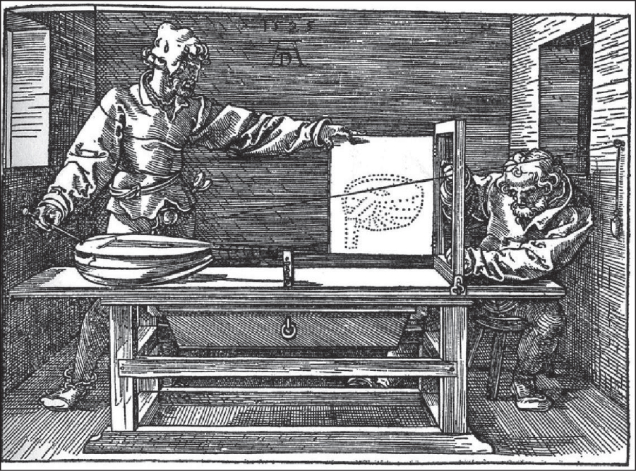
The apparatus consists of just a few parts. First, there is a long string that starts at the tip of a small pointer, passes through a screw eye attached to a wall, and ends at a small weight that maintains tension in the string. The pointer can be moved around by one person to touch various spots on an object to be drawn.
Second, there is a rectangular frame, with a board, which we’ll call the shutter, attached to it by a hinge so that the board can be moved aside (as shown in the woodcut) or rotated to cover the opening, as a shutter covers a window. On the board is mounted a piece of paper on which the drawing is to be made. In the woodcut, you can see a drawing of a lute partially made on the paper. The first man has moved the pointer to a new location on the lute itself. The string passes through the frame, and at the point where it does so, the second man holds a pencil. The string is pushed aside, the shutter is closed, and the pencil makes a new mark on the paper. This process is repeated until the whole drawing (in the form of many pencil marks) emerges. The man holding the pencil must hold it very steady for this to work, of course!
The result is a drawing of the lute consisting of many pencil marks on the paper, which can be connected together to make a more complete drawing. The drawing is a perspective view of the lute, showing the way the lute would look to a viewer whose eye was at the exact point where the string passes through the screw eye on the wall. Note that the height of the screw eye on the wall and the position of the table can both be changed, so the relative positions of the viewpoint and the drawing should be regarded as parameters of this scene-rendering engine.
The drawing’s fidelity can be attributed to three main factors. First, light travels along straight lines, so the stretched string represents a light path from the lute to the eye. Second, the drawing of the lute sits in the scene, and when the shutter is closed, it too sends light to the eye, from a corresponding direction. The points of high contrast in the scene are represented by marks in the drawing, which are themselves points of high contrast. Third, our visual system seems to “understand” a scene largely in terms of high-contrast edges in the scene, so marks on the paper and the real-world scene tend to provoke related responses in our visual systems.
Notice that the string always passes through the frame. If the first man moves the pointer to a place that cannot be seen from the screw eye through the frame, the string will touch the frame itself and bend around it. In this case, no mark is made on the paper.
We’ll now make our description of this “rendering” process slightly more formal, as shown in Listing 3.1.
Listing 3.1: Pseudocode for the Dürer perspective rendering algorithm.
1 Input: a scene containing some objects, location of eye-point
2 Output: a drawing of the objects
3
4 initialize drawing to be blank
5 foreach object o
6 foreach visible point P of o
7 Open shutter
8 Place pointer at P
9 if string from P to eye-point touches boundary of frame
10 Do nothing
11 else
12 Hold a pencil at point where string passes through frame
13 Hold string aside
14 Close shutter to make pencil-mark on paper
15 Release string
Three aspects of this algorithm deserve note, all within the loop that iterates over all points. First, the iteration is over visible points, so determining visibility will be important. Second, there may be an infinite number of visible points. Third, we’ve said what to do in the event that the string hits the frame rather than passing through the open area bounded by the frame. This is sure to happen if the object is so large that only a part of it is visible from the screw eye through the frame.
We’ll discuss the first issue presently; the second is addressed by agreeing to make an approximate rendering, which we do by selecting only a finite number of points, but choosing them so that the marks on the paper end up representing the shape well. The process of choosing a finite number of computations to perform, in order to best approximate a result that in theory requires an infinite number of computations, is critical, and will arise in many places in this book. In this chapter, we’ll render an object that is so simple that we can set this problem aside for the time being.
The third issue—avoiding drawing points that are outside the view—is also representative of a common operation in graphics. Generally, the process of avoiding wasting time on things outside the view region (the part of the world that the eye or camera can see) is called clipping. Clipping may be as simple as observing that a point (or a whole object) is outside the view region, or it may involve more complex operations, like taking a triangle that’s partly outside the view region and trimming it down until it’s a polygon completely inside the view region. For now, we’ll use a very simple version of clipping that’s appropriate for points only—we’ll just ignore points that are outside the view region.
We’ve made one useful simplification: To determine whether the tip of the pointer is inside the view region (a 3D volume), we check whether the place where the string passes through the frame is within the paper area (rather than the string touching the frame). The two tests are equivalent, but when it comes to implementing them, doing a point-in-rectangle test is easier than doing a point-in-3D-volume test.
Imagine that you can move the lute in Dürer’s woodcut.
a. How could you move it to ensure that “touches boundary of frame” is true for each iteration of the inner loop, thus resulting in almost all the work of the algorithm (aside from setup costs) falling into that clause?
b. How would you move it to ensure that no work fell into that clause?
(Your answers should be of the form “Move it closer to the frame and lift it up a little,” i.e., they should describe motions of the lute within the room.)
Imagine that, instead of moving the pointer at the end of the string to points on the lute and then seeing where they pass through the paper, the two men start with a piece of graph paper. For each square on the graph paper, the man with the pencil holds it at the center of the square; the shutter is then opened, and the man with the pointer moves it so that the string passes by the pencil point and so that the end of the string is touching either the lute, or the table, or the wall. The object being touched is noted, and when the shutter is closed again, the man with the pencil fills in the grid square with some amount of pencil-shading, corresponding to how dim or bright the touched point looks: If it appears dark, the grid square is filled in completely. If it’s light, the grid square is left empty. If it’s somewhere between light and dark, the grid square is shaded a light grey tone. Think for yourself for a moment about what kind of picture this produces. This approach (working “per pixel” and finding out what’s seen through that pixel) is the essence of ray tracing, as discussed in Chapter 14. A slightly different version of this approach, also developed by Dürer, is shown in Figure 3.2: The graph paper is on the table; the corresponding grid in the shutter consists of wires stretched across the shutter, or semitransparent graph paper, and the string and pointer are replaced by the line of sight through a small hole in front of the artist.

The renderings produced by the string-and-pointer method and the graph-paper method are quite different. The first produces an outline of the shapes in the scene (provided the first man chooses his points wisely). The second ignores the scene completely in choosing what to draw, and merely assigns a grayscale value to each grid square. In the event that the scene is very simple—that there are few outlines in the scene—the first method is quite fast. If the scene is very complex (imagine it consists of a bowl full of spaghetti!), then the second method, with its fixed number of grid squares, is faster. Of course, it’s only faster because we can, in the physical world, determine which point is visible instantaneously, which we’ll discuss further in the next section. In general, though, many techniques in graphics involve tradeoffs that are determined by scene complexity; this is just the first we’ve encountered.
Now that we have an understanding of this basic rendering process, how can we modernize it so that it becomes useful in computer graphics? We’ll focus on creating the drawing, or, more accurately, we’ll create a program that models this method of rendering. Through this, we hope you’ll gain insight into the ways we represent the real world in computer graphics. We start with a discussion of visibility.
3.2. Visibility
The matter of selecting only visible points might not even have occurred to Dürer, but it is important for us. One way for Dürer to determine whether a point P is visible is to place the pointer on P and see whether the string runs in a straight line to the screw eye, or has to bend around some other part of the lute or other object to get there. In making our simplified model of the process, we’ll disregard the issue of visibility determination, for the time being, not because it’s unimportant—Chapter 36 is entirely about data structures for improving visibility computations—but because it is both tricky in general and unnecessary for the model we’ll be drawing in this simple renderer.
3.3. Implementation
To mimic the woodcut’s algorithm, we’ll use algebra and geometry, and a very simple description of a very simple shape: We’ll describe a cube by giving the locations of its six corners (or vertices), and by noting which pairs of vertices are connected by an edge. Thus, our model of a cube can be considered a wire-frame model, in which an object is created by connecting pieces of wire together.
To make the geometry simple, we’ll establish a particularly nice way of measuring coordinates in the room. The origin of our coordinate system (see Figure 3.3) will be at the screw eye on the wall, and will be denoted E (for “eye”). The drawing frame will be in the z = 1 plane (i.e., we measure the distance from the screw eye to the plane of the drawing frame, and choose a system of units in which this distance is 1). The point on this plane that’s closest to the screw eye will be called T; its coordinates are (0, 0, 1). We’ll make the y-axis vertical and the x-axis horizontal, as shown.
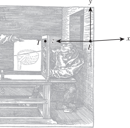
Figure 3.3: The coordinate system for the Dürer woodcut: The origin is at the screw eye, labeled E, and the y- and z-coordinate axes are shown there. The picture frame lies in the plane z = 1, parallel to the plane of the wall, z = 0. The x-coordinate arrow is horizontal, lying in the plane of the wall, approximately in the direction of the shading lines on the wall, while the z-coordinate arrow is horizontal and perpendicular to the wall. Due to the effects of perspective, the x-direction and z-direction appear almost parallel, but pointing in opposite directions, at the screw eye. The point T is the point in the frame of the drawing plane (z = 1) closest to the screw eye. The z-direction points from the screw eye toward T, making the xyz-coordinates of T be (0, 0, 1).
The frame, within the z = 1 plane, will extend from the point (xmin, ymin, 1) to the point (xmax, ymax, 1), where xmin < xmax and ymin < ymax, as the names suggest, and where, for simplicity and consistency with the drawing (in which the frame appears fairly square1), we’ll assume that the width, xmax – xmin, is the same as the height, ymax – ymin. To be precise, two opposite corners of the frame are points whose 3D coordinates are (xmin, ymin, 1) and (xmax, ymax, 1).
1. The panel that fills the frame does not appear square, however; we’ll stick with squareness for simplicity.
We’ll also imagine that the paper that fills the frame (when the shutter is closed) is actually graph paper, whose lower-left corner is labeled (xmin, ymin) and whose upper-right corner is labeled (xmax, ymax), therefore providing us with coordinates within the plane of the paper. Thus, to every 3D point (x, y, 1) whose last coordinate is 1, we have associated graph-paper coordinates (x, y).
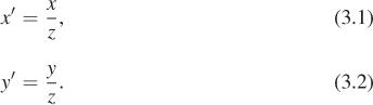
Now let’s suppose that we observe a point P = (x, y, z) of our object, as shown in Figure 3.4; the line from P to E (the string) passes through the frame at a point2 P′ = (x′, y′, z′). We need to determine the coordinates (x′, y′, z′) from the known coordinates x, y, and z.
2. The use of P and P′ to denote a point and another point associated to it can be very helpful in keeping the association in mind; unfortunately, most programming languages disallow the use of primes and other such marks in variable names, so in our code, we must use a different convention.
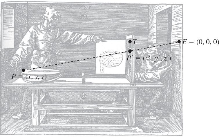
Figure 3.4: The point P = (x, y, z) is on our object. The string from P to the eye, E, will pass through the window frame at some location P′ = (x′, y′, z′). Note that z′ = 1, because we chose our coordinates to make that happen.
In Figure 3.5, we’ve drawn two similar triangles in the x = 0 plane. The vertices of the red triangle are (1) the point E = (0, 0, 0), (2) the projection of P′ onto the x = 0 plane, which is (0, y′, 1), and (3) the point (0, y′, 0), just below E. The vertices of the blue triangle are (1) the point E, (2) the projection of P onto the x = 0 plane, which is (0, y, z), and (3) the point (0, y, 0) well below E.
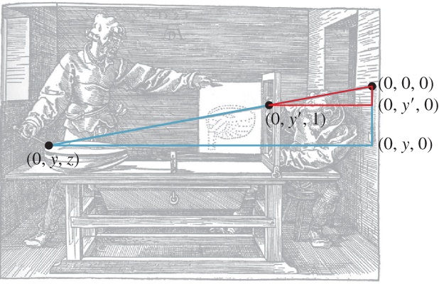
Figure 3.5: Two similar triangles overlaid on the picture in the x = 0 plane. The vertical edges of the small red and large blue triangles have lengths y′ and y, respectively. What are the lengths of their horizontal edges?
Similarity tells us that the ratio of the vertical to the horizontal side in the two triangles must be equal, that is, y′/1 = y/z. A similar argument, using triangles in the y = 0 plane (best visualized by imagining a bird’s-eye view of the scene), shows that x′/1 = x/z, which can be simplified to give
We now know how to find the coordinates of P′ from those of P in general! So we can describe our revised algorithm as shown in Listing 3.2.
Listing 3.2: Simple-implementation version of the Dürer rendering algorithm.
1 Input: a scene containing some objects
2 Output: a drawing of the objects
3
4 initialize drawing to be blank
5 foreach object o
6 foreach visible point P =(x,y,z) of o
7 if xmin≤(x/z)≤xmax and ymin ≤ (y/z) ≤ ymax
8 make a point on the drawing at location (x/z, y/z)
Let’s pause for a moment to examine this: We’ve now got the x- and y-coordinates of the pencil marks in the picture plane. But if we are to view the eventual picture from the location of the screw eye in the wall, the direction of increasing x will point to our left. (The direction of increasing y will still point up, as expected.) We could choose to plot our points on a piece of graph paper in which we decide that x increases to the left, or we can flip the sign on x to make it increase to the right. We’ll do the latter, because it’s consistent with the more general approach we’ll take later. So we revise the last part of our algorithm to the code shown in Listing 3.3.
Listing 3.3: Minor alteration to the Dürer rendering algorithm.
1 if xmin ≤(x/z)≤xmax and ymin≤(y/z)≤ ymax
2 make a point on the drawing at location (-x/z, y/z)
To complete our modern-day implementation, we need (1) a scene, (2) a model of the objects in the scene, and (3) a method for drawing things.
For simplicity, our scene will consist of a single cube. Our model of the cube will initially consist of a set containing the cube’s eight vertices. A basic cube can be described by the following table:
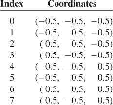
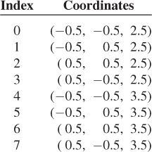
Unfortunately, this cube is centered on the eyepoint, rather than being out in the area of interest, beyond the frame. By adding 3 to each z-coordinate, we get a cube in a more reasonable location:
3.3.1. Drawing
The vertices of a cube are indeed interesting points, but we should draw points from all over the surface of the cube to really mimic Dürer’s drawing. On closer inspection, however, we see that the points selected by the two apprentices lie on what we could call “important lines” like the outline of the lute, or sharp edges between pairs of surfaces.3 For the cube, these important lines consist of all the points on the edges of the cube. Drawing all these points (or even a large number of them) might be needlessly computationally expensive; fortunately, there’s a way around this expense: If A and B are vertices with an edge between them, and we project A and B to points A′ and B′ in the drawing, then we can see that the points between A and B will project to points on the line segment between A′ and B′. We could verify this geometrically, or simply rely on the familiar experience that photographs of straight lines always appear straight.4 So, instead of finding many points on the edge and drawing them all, we’ll simply compute A′ and B′ and then draw a line segment between them.
3. The question of which lines in a scene are important is of considerable interest in nonphotorealistic or expressive rendering, as discussed in Chapter 34.
4. For cameras with high-quality, nondistorting lenses anyhow!
The preceding paragraph suggests that we can say that “Perspective projection from space to a plane takes lines to lines” or “takes line segments to line segments.” Think carefully about the first claim and find a counterexample. Hint: Is our perspective projection defined for every point in space?
A word to the wise: The sorts of subtleties you discovered in this exercise are not mere nitpicking! They are the kinds of things that lead to bugs in graphics programs. Because graphics programs tend to operate on a great deal of data, nearly every possible part of a program will often be tested in a sample execution. Thus, bugs that might survive testing on a less demanding system will often reveal themselves early in graphics programs.
For those who did not come up with counterexamples, we give them here. First, for a line that passes through the eye, the perspective projection is not even defined for the eyepoint. And the non-eyepoints of the line project to a single point rather than to an entire line. If we agree to ignore points at which the projection is undefined, there’s a further problem: The eye is at location (0, 0, 0), and the projection plane is parallel to the xy-plane. This means that any line segment that passes through the z = 0 plane contains a point that cannot be projected. The projection of such a segment will consist of two separate pieces. Convince yourself of this by projecting the segment from (![]() , 0,1) to (
, 0,1) to (![]() , 0, –1) onto the z = 1 plane by hand.
, 0, –1) onto the z = 1 plane by hand. ![]() In the language of projective geometry, “perspective projection takes extended lines to extended lines, except that it is undefined on the pencil of lines containing the projection point.”
In the language of projective geometry, “perspective projection takes extended lines to extended lines, except that it is undefined on the pencil of lines containing the projection point.”
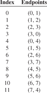
Returning to our program, we enhance our model of the cube to include a list of edges, described by the vertex indices of their endpoints:
This enhanced model is shown in Figure 3.6.
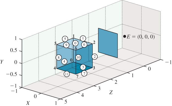
Figure 3.6: The labels for the vertices and edges of our cube model. Edge indices are in circles. The eyepoint and frame from the Dürer woodcut are also included, although we have chosen to adjust their relative positions by placing the frame in this case so that it extends from – ![]() to
to ![]() in both x and y. Thus, we’re viewing the cube “at eye level” rather than “from above,” as Dürer viewed the lute.
in both x and y. Thus, we’re viewing the cube “at eye level” rather than “from above,” as Dürer viewed the lute.
Now let’s determine a method for drawing this enhanced representation. To update our algorithm to a version that draws lines, we have to make a choice. Do we iterate through the edges, and for each edge, compute where its endpoints project, and then connect them with a line? Or do we iterate through the vertices first, computing where each vertex projects, and then iterate through the edges, using the precomputed projected vertices? Since each vertex is shared by three edges, the first strategy involves three times as many projection computations; the second involves three times as many data-structure accesses. For such a small model, the performance difference is insignificant. For larger models, these are important tradeoffs; the “right” answer can depend on whether the work is done in hardware or in software, and if in hardware, the precise structure of the hardware, as we’ll see in later chapters. We’ll use the second approach, but the first is equally viable. The results of this approach to rendering the cube are shown in Figure 3.7, both in 3-space and in the plane of the frame.
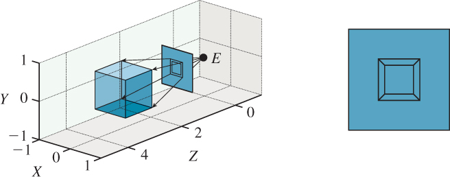
Figure 3.7: The result of the rendering algorithm, (a) shown in place (i.e., drawn in the frame), with rays from the eye to the four near corners of the cube shown, projecting those corners onto the picture plane, and (b) seen directly, with the surrounding square (which ranges from – ![]() to
to ![]() in both x and y) drawn to give context.
in both x and y) drawn to give context.
Furthermore, there’s another problem: When we were transforming only points, we could perform clipping on a point-by-point basis. But now that we plan to draw edges, we have to do something if one endpoint is inside and the other is outside the frame. We’ll ignore this problem, and assume that if we ask our graphics library to draw a line segment in our picture, and the coordinates of the line segment go outside the bounds of the picture, nothing gets drawn outside the bounds. (This is true, for example, for WPF.) A preliminary sketch of the program is given in Listing 3.4.
Listing 3.4: Edge-drawing version of the Dürer rendering algorithm.
1 Input: a scene containing one object ob
2 Output: a drawing of the objects
3
4 initialize drawing to be blank;
5 for (int i = 0; i < number of vertices in ob; i++){
6 Point3D P = vertices[i];
7 pictureVertices[i] = Point(-P.x/P.z, P.y/P.z);
8 }
9 for {int i = 0; i < number of edges in ob; i++){
10 int i0 = edges[i][0];
11 int i1 = edges[i][1];
12 Draw a line segment from pictureVertices[i0]
13 to pictureVertices[i1];
14 }
Finally, we have to observe that this algorithm depends on the “picture rectangle” having coordinates that run from (xmin, ymin) to (xmax, ymax). We can, however, remove this dependency by using coordinates that range from 0 to 1 in both directions, as is very common in graphics libraries. We can convert the x-coordinates as follows. First, subtract xmin from the x-coordinates; the new coordinates will range from 0 to xmax – xmin. Then divide by xmax – xmin, and the new coordinates will range from 0 to 1. So we have
an analogous expression gives us y-values that range from 0 to 1. Because we’ve required that xmax – xmin = ymax – ymin, we get no distortion by transforming x and y this way: Both are divided by the same factor. The program, modified to include this transformation, is shown in Listing 3.5.
Recall that we negated x so that the picture would be correctly oriented. When we negate xnew, however, the resulting values will range from –1 to 0. We therefore add 1 to return the result to the range 0 to 1, in line 11 of Listing 3.5.
Listing 3.5: Edge-based implementation with the limits of the view square included as parameters.
1 Input: a scene containing one object o, and a square
xmin≤ x ≤xmax and ymin ≤y≤ymax in the z = 1 plane.
2 Output: a drawing of the object in the unit square
3
4 initialize drawing to be blank;
5 for(int i= 0; i < number of vertices in o; i++){
6 Point3D P = vertices[i];
7 double x = P.x/P.z;
8 double y = P.y/P.z;
9 pictureVertices[i] =
10 Point(1 - (x - xmin)/(xmax - xmin),
11 (y - ymin)/(ymax - ymin));
12 }
13 for{int i ≤ 0; i < number of edges in o; i++){
14 int i0 ≤ edges[i][0];
15 int i1 ≤ edges[i][1];
16 Draw a line segment from pictureVertices[i0] to
17 pictureVertices[i1];
18 }
These zero-to-one coordinates are often called normalized device coordinates: They can be thought of as describing a fraction of the left-to-right or top-to-bottom range of a display device; if the display device isn’t square, then a coordinate of 1. 0 represents the smaller of the two dimensions. A typical desktop monitor might have vertical coordinates that range from 0 to 1, but horizontal coordinates that range from 0 to 1. 33.
The normalization process—converting from the range [xmin, xmax] to the range [0, 1]—occurs often; it’s worth memorizing the form of Equation 3.3.
Verify, in Listing 3.5, that a vertex that happens to be located at the lower-left corner of the view square, that is, (xmin, ymin, 1), does indeed transform to the lower-left corner of the final picture, that is, the corresponding pictureVertex is (0, 1); similarly, verify that (xmax, ymax, 1) transforms to (1, 0).
3.4. The Program
We’ll use a simple WPF program, based on a standard test bed described extensively in the next chapter, to implement this algorithm. The resultant program is downloadable from the book’s website for you to run and to experiment with. For this application, the critical elements of the test bed are the ability to create and display dots (small disks that indicate points) and segments (line segments between dots) on a Canvas that we call the GraphPaper. Positions on our graph paper are measured in units of millimeters, which are more readily comprehended than WPF default units, which are about ![]() of an inch. To make the drawing a reasonable size, we’ll multiply our algorithmic results (coordinates ranging from zero to one) by 100. The important parts of the program are shown in Listing 3.6, with elisions indicated by
of an inch. To make the drawing a reasonable size, we’ll multiply our algorithmic results (coordinates ranging from zero to one) by 100. The important parts of the program are shown in Listing 3.6, with elisions indicated by [...].
Before you examine the code, though, we’ll warn you that this use of WPF is very different from what you saw in Chapter 2. In that chapter, we demonstrated the declarative aspects of WPF that are easy to expose through XAML. The test bed uses these declarative aspects to build a window, some menus, and controls, and to lay out the GraphPaper on which we’ll do our drawing. But the production of actual pictures within the GraphPaper is all done in C#. That’s because for most of the programs we’ll want to write, expressing things in XAML is either cumbersome or impossible (not every feature of WPF is exposed through XAML). In general, it makes sense to use the declarative specification whenever possible, especially for layout and for data dependencies, and to use C# whenever substantial algebraic manipulations may be needed.
Listing 3.6: C# portion of the implementation of the Dürer algorithm.
1 public Window1()
2 {
3 InitializeComponent();
4 InitializeCommands();
5
6 // Now add some graphical items in the main Canvas,
7 whose name is "Paper"
9 gp = this.FindName("Paper") as GraphPaper;
10
11 // Build a table of vertices:
12 int nPoints = 8;
13 int nEdges = 12;
14
15 double[,] vtable = new double[nPoints, 3]
16 {
17 {-0.5, -0.5, 2.5}, {-0.5, 0.5, 2.5},
18 {0.5, 0.5, 2.5}, ...};
19 // Build a table of edges
20 int [,] etable = new int[nEdges, 2]
21 {
22 {0, 1}, {1, 2}, ...};
23
24 double xmin = -0.5; double xmax = 0.5;
25 double ymin = -0.5; double ymax = 0.5;
26
27 Point [] pictureVertices = new Point[nPoints];
28
29 double scale = 100;
30 for (int i = 0; i < nPoints; i++)
31 {
32 double x = vtable[i, 0];
33 double y = vtable[i, 1];
34 double z = vtable[i, 2];
35 double xprime = x / z;
36 double yprime = y / z;
37
38 pictureVertices[i].X = scale * (1 - (xprime - xmin) /
39 (xmax - xmin));
40 pictureVertices[i].Y = scale * (yprime - ymin) /
41 (ymax - ymin);
42 gp.Children.Add(new Dot(pictureVertices[i].X,
43 pictureVertices[i].Y));
44 }
45
46 for (int i = 0; i < nEdges; i++)
47 {
48 int n1 = etable[i, 0];
49 int n2 = etable[i, 1];
50
51 gp.Children.Add(new Segment(pictureVertices[n1],
52 pictureVertices[n2]));
53 }
54
55 ...
56 }
We begin with a few comments. First, the code is not at all efficient (e.g., there was no need to declare the variables x, y, and z), but it follows the algorithm very closely. For making graphics programs that are debuggable, this is an excellent place to start in general: Don’t be clever until your code works and you find that you need to be clever. Second, we’ve used names for all the important things that we might consider changing, like xmin and nEdges. That’s because most test programs like this one survive far longer than originally intended, and get altered for other uses; symbolic names help us communicate with our former selves (who wrote the program originally). Third, the program is not “software engineered”: We didn’t define a class to represent general shapes, for instance—we just used an array of a fixed size to represent one shape, the cube. That was deliberate. The program was meant to be used, experimented with, and thrown away (or perhaps reused in another experiment). The point of this program was to verify our understanding of a simple concept. It’s not a prototype for some large-scale project. Indeed, if you find yourself building something of even a modest scale atop this framework, you’re making a big mistake: The pieces of this framework were designed to make testing and debugging easy. If you run the program and place your cursor over one of the dots, for instance, a tool-tip will appear telling you the dot’s coordinates; the same goes for the edges. That makes sense when you’re debugging, but by the time you’re drawing 10,000 edges, it’s a huge amount of overhead. Remember that this framework is a test bed for experiments, and that all the code you write within it should be considered disposable. While this advice may seem contradictory—we’ve said to throw away code, but to code decently because you’ll be reusing it—it reflects our experience: Even code we intend to throw away does get reused, often for other throwaway applications! It’s worth investing a little time to make these future uses easier, but not worth investing so much that it takes hours to code up a simple idea and confirm your understanding.
The results are what we expect (see Figure 3.8): a perspective picture of a wireframe cube. We’ve created our first rendering! There’s clearly a long way to go from this to the kinds of special effects seen in video games and Hollywood films, but some of the important ideas—building a mathematical model, converting it to a 2D picture5—are present in our simple renderer in a basic form.
5. We’re using the term “picture” informally here, as in “something you can look at.”
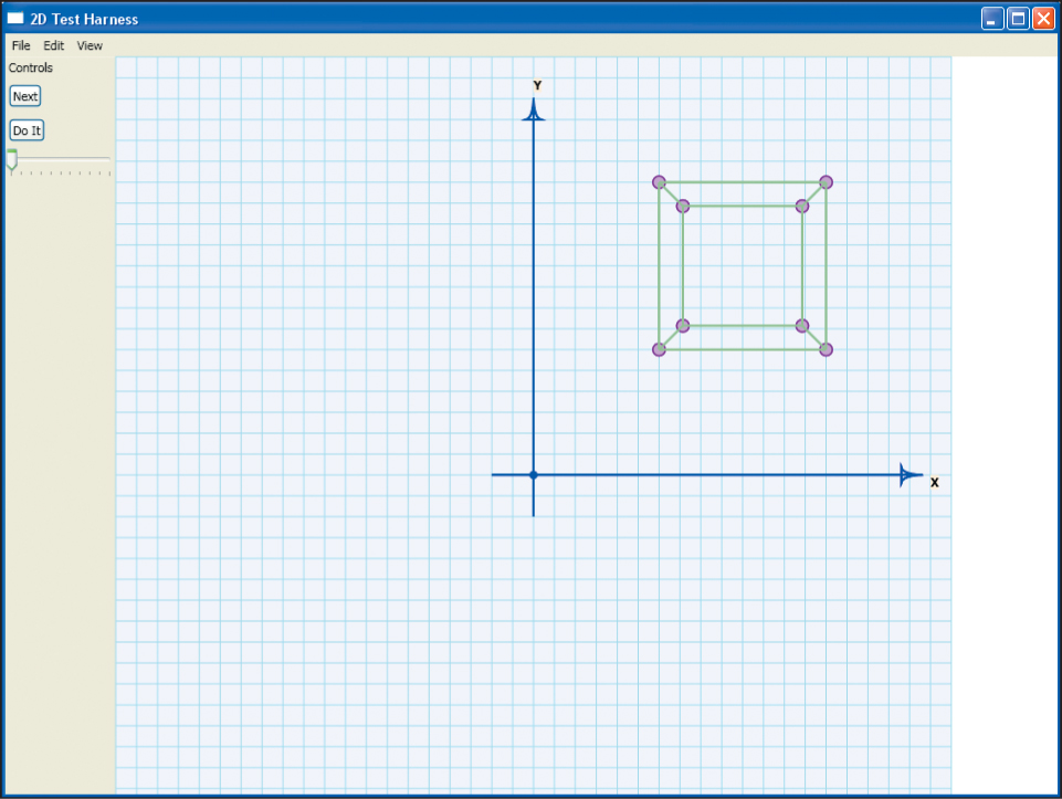
Figure 3.8: The result of the Dürer program: a wire-frame cube, shown in perspective, on a background that looks like graph paper. The axes on the graph paper are part of the GraphPaper itself, set up by the test bed, and are not drawn by the Dürer rendering part of the program.
3.5. Limitations
We will now step back and look critically at this success. When you run the program, you see a perspective view of a cube, consisting of 12 line segments (with dots at the corners of the cube as well), as expected.
There are several limitations to the program. First, the wire-frame drawing means that we can see both the back and the front of the cube. We could address this in much the same way we addressed the drawing of edges: We could observe that all points on a face of a cube (one of the square sides of the cube) will project to points in the quadrilateral defined by the projections of the four vertices. So, instead of keeping an edge table, we could keep a face table, and for each face, we could draw a filled polygon in two dimensions. (We could draw both faces and edges, of course.) Using this approach, our main concern will be to find a way to draw only polygons that face toward the eye rather than away from it. There are many strategies for doing this, but all of them require either more mathematics than we wish to introduce in this chapter, or more complex data structures than we wish to discuss at this time.
Second, although we all know that we see objects because of the light they emit (which enters our eyes and causes us to perceive something, as described in Chapters 5 and 28), there’s nothing in our current program that describes anything about light (except that our use of straight lines for projection is based on the understanding that light travels along straight lines). We would get the same picture of a cube whether we imagined any light being present or not. This also means that all kinds of other light-dependent features, like shadows and shaded parts of the surface, cannot manifest themselves. It’s possible to add these without an explicit model of light, but it’s a mistake to do so, according to the Wise Modeling principle.
Third, when this program runs, it only shows one model (the cube), and only shows it in one position. We did a lot of work for not much output; our program is not versatile enough to display other scenes without changing the code. This can be addressed by storing the data representing the cube in a file that can be read by the program; a typical representation would begin with a vertex count, a list of vertices, an edge count, and a list of edges. Although it’s less compact, it’s wise to make such files contain explicit tags on the data, and to allow comments; it will make debugging your programs much easier. Here’s an example file for representing a cube:
1 # Cube model by jfh
2 nVerts: 8
3 vertTable:
4 0 -0.5 -0.5 -0.5
5 1 -0.5 0.5 -0.5
6 ...
7 7 0.5 0.5 0.5
8 # Note that each edge of cube has length = 1
9
10 edgeTable:
11 0 0 1
12 1 1 2
13 ...
14 11 7 8
Other formats are certainly possible; indeed, there are many, many formats for specifying models of all sorts, and programs for interconverting them (sometimes losing some data in the conversion). Because the choice of formats is subject to the whims of fashion, and changes quickly, we’ll make no attempt to survey them.
With any such storage format, one can define multiple shapes, such as the cube, a tetrahedron, or even a faceted sphere, and enhance the program to load each one in turn, adding some variety. To do so will require that you understand the test bed more fully by reading parts of the next chapter, however.
We can also enhance the program by adding a limited form of animation: The xy-coordinates of the bottom (or top) four vertices of our cube are four equally spaced points on a circle of radius ![]() , namely r(cos θ, sin θ), where
, namely r(cos θ, sin θ), where ![]() , and
, and ![]() . We can create a slightly rotated cube by making
. We can create a slightly rotated cube by making ![]() , and
, and ![]() for the four corners, for some small value of t. By gradually increasing t, and redrawing the model each time, we can display a rotating cube.
for the four corners, for some small value of t. By gradually increasing t, and redrawing the model each time, we can display a rotating cube.
This method of explicitly changing the coordinates of the cube and then redisplaying it is not particularly efficient. The cube effectively becomes a parameterized model, with the rotation amount, t, serving as the parameter. The problem is that when we want to rotate the cube6 in the yz-plane instead of the xy-plane, we need to change the model. And if we want to rotate first in one plane, then in the other, we must do some messy algebra and trigonometry. It’s actually far simpler to model the cube just once, and then learn how to transform its vertices by a rotation (or other operations). We’ll discuss this extensively in the next several chapters.
6. We speak of rotation in the xy-plane rather than “around the z-axis,” because rotation in a plane generalizes to all dimensions, while rotation about an axis is specific to three dimensions. Chapter 11 discusses this further.
On the other hand, there are models that are defined parametrically, and are animated by changing these parameters. So-called “spline” models are a particularly important example, discussed in Chapter 22, but others abound, particularly in physical simulations: A model of fluid, for instance, has parameters like the viscosity and the density of the fluid, as well as the initial positions and velocities of the fluid particles. The effects of these parameters on the appearance of the fluid at some time are rather indirect—we have to perform a simulation to understand the effects—but it is a parameterized model nonetheless.
3.6. Discussion and Further Reading
The “rendering” in this chapter was a little unusual, in the sense that we converted our 3D scene into a collection of 2D things (points and lines), which we then drew with a 2D renderer. In this sense, the process somewhat resembles a compiler that turns a high-level language into low-level assembly language. Only when this assembly language is further processed into machine language and executed does the computation take place. In the same way, only when we actually draw the points and lines with WPF’s 2D rendering tools do we get a picture. Transformations like this into intermediate representations occur elsewhere in graphics as well. In some expressive rendering algorithms, input images are transformed into an intermediate representation that consists of edges detected by some image-processing algorithms and regions bounded by those edges, for instance. Choosing a good intermediate representation can make the difference between success and failure.
The discovery of perspective in Western art, and the working out of the associated mathematics, is a fascinating subject. When lines that are parallel in the world appear to converge in the rendered picture, the eye is drawn to the point of convergence, or vanishing point. Almost as fascinating as the development of perspective is the clever use by artists of this property of vanishing points; sometimes artists created different vanishing points for different regions of a picture, drawing the viewer’s eye to multiple things in the scene (The Resurrection, by Piero della Francesca, is said to have this property.) It’s not known whether this was in fact deliberate. There are many systematic ways of creating proper perspective renderings using so-called “vanishing points” and ideas from projective geometry. These too can be considered basic rendering engines like the one shown in the Dürer woodcut.
Also intriguing is the understanding one can gain of non-Western art. Rock’s book on perception [Roc95], for instance, explains that the view seen in some Chinese scroll paintings, which appears odd to the Western eye, is actually a perspective-correct view for a view from a very high point, with the projection plane perpendicular to the ground plane.
Perspective projections do not preserve relative lengths (think of a picture of railroad tracks disappearing into the distance—the equal distances between adjacent railroad ties become unequal distances in the picture), but they do preserve some other properties. The study of projections and the transformations of space that are associated to them became the field of projective geometry; for the mathematically curious, the books of Hartshorne [Har09]and Samuel [SL88] are excellent introductions.
Representations of polyhedral models by arrays of vertices together with arrays of faces described by vertex indices are sometimes called indexed face sets; a large repository of models stored in this way has been collected in the Brown Mesh Set [McG]. While not particularly compact, it is an easy-to-parse format. Similarly simple is the PLY2 format. Many example models are available on the Internet in both forms. More complex model formats, using more compact binary representations, abound. One fairly common format was 3DS, developed for use with the 3D Studio Max software (now known as 3ds Max), and widely adopted or imported by other tools. 3ds Max now uses the .max format, which is proprietary, but many 3DS models are still available. And Maya, another popular shape-modeling program, has its own proprietary format, .mb. Both are essentially meta-formats, which specify the plugin (shared library) that should be used to parse each subpiece of a model; in practice, it’s impractical to reverse-engineer such a format, and as a result, for hobbyist and classroom use people continue to use older and simpler formats.
What we called the “view region” in this chapter—the portion of the world that’s visible in the picture we’re making—is an instance of the more general notion of view volume; the difference is that a view volume, rather than being an infinite pyramid, may be truncated so that objects farther away than some distance are ignored, as are those closer than some other distance. These “near” and “far” distances can be adjusted to make some algorithms more efficient (by reducing the set of objects we need to consider during rendering) or more accurate (by using fixed-point arithmetic to more precisely represent a range of values). The general matter of defining a view volume is discussed extensively in Chapter 13.
3.7. Exercises
Exercise 3.1: Suppose that the apprentice holding the pencil in the Dürer drawing not only made a mark, but also wrote next to it the height (above the floor) of the weight at the end of the string. That number would be the distance from the eye to the object (plus some constant). Now suppose we make a first drawing-with-distances of a lute, whose owner then takes it home. We later decide that we’d really like to have a candlestick in the picture, in front of the lute (i.e., closer to the eye).
(a) If we place the candlestick on the now-empty table, but in the correct position, and make a second drawing-with-distances, describe how one might algorithmically combine the two to make a composite drawing showing the candlestick in front of the lute. This idea of depth compositing is one of many applications of the z-buffer, which you’ll encounter again in Chapters 14, 32, 36, and 38. The recording of depths at each point is rather like the values stored in a z-buffer, although not identical.
(b) Try to think of other things you might be able to do if each point of an image were annotated with its distance from the viewpoint.
Exercise 3.2: The dots at the corners of the rendered cube in Figure 3.8 appear behind the edges, which doesn’t look all that natural; alter the program to draw the dots after the segments so that it looks better. Alter it again to not draw the dots at all, and to draw only the segments.
Exercise 3.3: We can represent a shape by faces instead of edges; the cube in the Dürer program, for instance, might be represented by six square faces rather than the cube’s 12 edges. We could then choose to draw a face only if it faces toward the eye. “Drawing,” in this case, might consist of just drawing the edges of the face. The result is a rendering of a wire-frame object, but with only the visible faces shown. If the object is convex, the rendering is correct; if it’s not, then one face may partly obscure another. For a convex shape like a cube, with the property that the first two edges of any face are not parallel, it’s fairly easy to determine whether a face with vertices (P0, P1, P2, ...) is visible: You compute the cross product7 w = (P2 –P1) × (P1 –P0) of the vectors, and compare it to the vector v from the eye, E, to P0, that is, v = P0 –E. If the dot product of v and w is negative, the face is visible. This rule relies on ordering the vertices of each face so that the cross product w is a vector that, if it were placed at the face’s center, would point into free space rather than into the object.
7. We review the dot product and cross product of vectors in Chapter 7.
(a) Write down a list of faces for the cube, being careful to order them so that the computed “normal vector” w for each face points outward.
(b) Adjust your program to compute visibility for each face, and draw only the visible faces.
(c) The cross- and dot-product based approach to visibility determination described in this exercise fails for more complex shapes, but later in the book we’ll see more sophisticated methods for determining whether a face is visible. For now, give an example of an eyepoint, a shape, and a face of that shape with the property that (i) the dot product of v and w is negative, and (ii) the face is not visible from the eye. You may describe the shape informally. Hint: Your object will have to be nonconvex!
Exercise 3.4: As in the preceding exercise, we can alter a wire-frame drawing to indicate front and back objects in other ways. We can, for instance, consider all the lines of the object (the edges of the cube, in our example) and sort them from back to front. If two line segments do not cross (as seen from the viewpoint) then we can draw them in either order. If they do cross, we draw the one farther from the eye first. Furthermore, to draw a line segment (in black on a white background), we first draw a thicker version of the line segment in white, and then the segment itself in black at ordinary thickness. The result is that nearer lines “cross over and hide” farther lines.
(a) Draw an example of this on paper, using an eraser to simulate laying down the wide white strip.
(b) Think about how the lines will appear at their endpoints—will the white strips cause problems?
(c) Suppose two lines meet at a vertex but not at any other point. Does the order in which they’re drawn matter? This “haloed line” approach to creating wire-frame images that indicate depth was used in early graphics systems [ARS79], when drawing filled polygons was slow and expensive, and even later to help show internal structures of objects.
Exercise 3.5: Create several simple models, such as a triangular prism, a tetrahedron, and a 1 × 2 × 3 box, and experiment with them in the rendering program.
For the final two exercises, you may need to read parts of Chapter 4.
Exercise 3.6: Enhance the program by adding a “Load model” button, which opens a file-loading dialog, lets the user pick a model file, loads that model, and makes a picture of it.
Exercise 3.7: Implement the suggestion about displaying a rotating cube in the program. Add a button that, when the cube is loaded, can update the locations of the cube vertices by computing them with a new value of t, the amount to rotate. To make the animation look smooth, try changing t by .05 radians per button click.