20.5 MATRIX TRIANGULARIZATION ALGORITHM

This section shows the algorithm to convert a square matrix A to an upper triangular matrix U. Once we obtain a triangular matrix, we can use forward or back substitution to solve the system of equations.

Assume we are given the system of linear equations described by

(20.26)

The solution for this system will not change if we premultiply both sides by the Givens matrix G_pq:

(20.27)

Premultiplication with the Givens matrix transforms the linear system into an equivalent system

(20.28)

and the solution of the equivalent system is the same as the solution to the original system. This is due to the fact that premultiplication with the Given matrix performs two elementary row operations:

Let us assume we have the following system of linear equations

(20.29)

To solve this system, we need to convert the system matrix to an upper triangular matrix. So we need to change element a_2,1 from 3 to 0. After multiplying by the Givens matrix G₂₁, element is given by the equation

(20.30)

Therefore, we have

(20.31)

For our case we get tan θ = 3/1 and θ = 71.5651°. The desired Givens matrix is given by

(20.32)

The transformed system becomes

(20.33)

The solution to the system is x = [−4 4]^t.

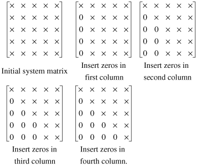
Givens rotations can be successively applied to the system matrix to convert it to an upper triangular matrix as shown in the following steps.

Assume our system matrix is 5 × 5 as shown below where the symbols × indicate the elements of the matrix.

20.5.1 Givens Rotation Algorithm

We now show the algorithm that converts the system matrix to an upper triangular matrix so that back substitution could be used to solve the system of linear equations. Algorithm 20.1 illustrates the steps needed. We can see that the algorithm involves three indices i, j, and k and the graph technique of Chapter 10 might prove difficult to visualize. However, the graph technique is useful as a guideline for the more formal computation geometry technique of Chapter 11.

Since estimation of rotation angle θ_ik is outside the innermost loop, we choose to have it estimated separately. In the discussion below, we ignore estimation of the rotation angle and concentrate on applying the rotations.

Algorithm 20.1 is three-dimensional (3-D) with indices 1 ≤ k < N, k < i ≤ N, and k ≤ j ≤ N. Thus, the convex hull defining the computation domain is pyramid-shaped as shown in Fig. 20.4. The figure shows bird’s eye and plan views of the pyramid shaped or layered structure of the dependence graph for the matrix triangularization algorithm when system matrix has dimensions 5 × 5.

Figure 20.4 Bird’s eye and plan views of the pyramid-shaped or layered structure of the dependence graph for the matrix triangularization algorithm when system matrix has dimensions 5 × 5.

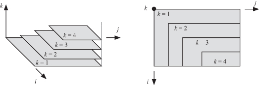
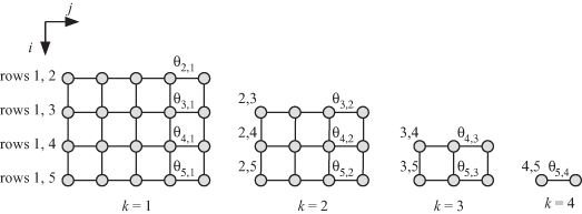
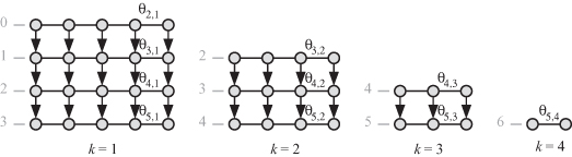
Figure 20.5 shows the details of the dependence graph on a layer-by-layer basis when system matrix has dimensions 5 × 5. This way we can think of the dependence graph in terms of multiple two-dimensional (2-D) dependence graphs that are easier to visualize. We see that variable θ_ik is propagated along the j direction. Variable a_kj is propagated along the i direction. This variable represents an element of the top row in each iteration, which is used by the lower rows to apply the Givens rotations.

Figure 20.5 Dependence graph for the matrix triangularization algorithm when system matrix has dimensions 5 × 5.

20.5.2 Matrix Triangularization Scheduling Function

The scheduling vector s assigns a time index value to each point in our computation domain as

(20.34)

The reader will agree that a 3-D computation domain is difficult to visualize and to investigate the different timing strategies. However, there are few observations we can make about the components s_1, s₂, and s₃.

At iteration k, a node at row i + 1, for example, a node at location (i + 1, j, k), is proceed after node (i, j, k) has been evaluated. Thus, we have

(20.35)

(20.36)

At iteration k, once the rotation angle has been evaluated, all the matrix elements in the same row can be processed in any order. Thus, we have

(20.37)

(20.38)

The rotation angle at iteration k + 1 uses the node at location (k + 2, k + 1, k). This angle estimation can proceed after node at location (k + 2, k + 1, k) has been processed. Thus, we have

(20.39)

(20.40)

We can choose three possible scheduling vectors while satisfying the above observations:

(20.41)

(20.42)

(20.43)

Perhaps the simplest scheduling function to visualize is s₂. The DAG for this function for the case of a 5 × 5 system is shown in Fig. 20.6. The figure shows the different layers separately for clarity.

Figure 20.6 DAG diagram for a 5 × 5 system for s₂ scheduling function.

We can see from the figure that the work done at each time step starts at a value N for the first two time steps then increases to 1.5N for time steps 2 and 3 and so on.

20.5.3 Matrix Triangularization Projection Direction

Based on the three possible scheduling functions discussed in the previous section, we are able to choose appropriate projection directions. Possible simple projection vectors are

(20.44)

(20.45)

(20.46)

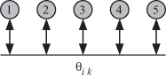
For illustration, let us choose s₂ and d₁. The reduced DAG () is shown in Fig. 20.7. This choice of projection direction produces a column-based implementation since each thread or PE operates on a column of the system matrix. The rotation angle θ_ik is broadcast to all the threads or PEs. At iteration k thread T_k or PE_k is responsible for generating N − k rotation angles and propagating these angles to all the threads or PEs to its right side.

Figure 20.7 Reduced DAG diagram for a 5 × 5 system for s₂ scheduling function and d₁ projection direction.