
CHAPTER 46
VaR: Alternative Measures
Aims
- To examine non-parametric methods of estimating VaR such as historical simulation and bootstrapping procedures.
- To demonstrate how Monte Carlo simulation (MCS) is used to estimate VaR for portfolios containing options.
- To analyse variants on the traditional VaR approach such as stress-testing and extreme value theory.
46.1 HISTORICAL SIMULATION
When using the variance-covariance method to calculate portfolio-VaR, we assume returns are normally distributed – hence we can use the ‘1.65’ scaling factor in our VaR calculations (for the 5th percentile). But if returns are actually non-normal using ‘1.65’ is no longer valid and it would produce biased forecasts of VaR. Historical simulation (HS), directly uses actual historical data on returns to calculate VaR and does not assume a particular distribution for returns – we take whatever distribution is implicit in the historical data.
When we use the variance-covariance approach to measure risk we explicitly measure the variance (standard deviation) and the covariances (correlations) between each of the asset returns in our portfolio. These variance and covariances (correlations) are ‘parameters’. However, in the HS approach, variances and covariances are not explicitly estimated – hence the term ‘non-parametric’. Instead these features of the data are ‘encapsulated’ in the time path of actual returns used in the HS approach.
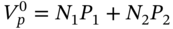
The HS approach is straightforward and intuitive. Consider Figure 46.1, which shows daily returns over the past 1,000 days on two stocks, which could be AT&T and Exxon. In Figure 46.1 there are only a few representative numbers visible (out of the 1,000) but you can still make an informed guess about what these figures are telling you about volatilities and correlation. For example, approximately, what is the mean daily return of stock-1 and stock-2 and their standard deviations, and do the latter look as if they are changing over time? Very approximately the mean daily return on both stocks could be zero. The standard deviation of stock-1 looks to be around 2% per day and is fairly constant over time. For stock-2 the average volatility is somewhat higher and its volatility clearly varies over time, starting low in the early periods at around 1.5% and rising to quite a high level on days 701–3.
| Currently hold $100 in each of 2 stocks | ||||||||||
| Day | 1 | 2 | 3 | … | 700 | 701 | 702 | 703 | … | 1,000 |
| R 1 (%) | +2 | +1 | +4 | … | −3 | −2 | −1 | −1 | +2 | |
| R 2 (%) | +1 | +2 | 0 | … | −1 | −5 | −6 | +15 | −5 | |
| dVp($) | +3 | +3 | +4 | … | −4 | −7 | −7 | +14 | −3 | |
| Order the 1,000 values for the $-change in portfolio value in ascending order −12, −11, −11, −10, −9, −9, −8, −7, −7, −6 || −5, −4, −4, …, 0, +2, +3, +3, +4, +5, …, +8, …, +14 VaR forecast for tomorrow at 1% tail (10th most negative) = −$6 |
||||||||||
FIGURE 46.1 Historic simulation
Next, by looking across the row ‘![]() ’, we can describe the time series properties of the returns on stock-1. When stock-1 has positive returns they tend to stay positive for a while and when they become negative there is a tendency for them to remain negative – this means that stock returns R1 are not independent over time – they are autocorrelated.1
’, we can describe the time series properties of the returns on stock-1. When stock-1 has positive returns they tend to stay positive for a while and when they become negative there is a tendency for them to remain negative – this means that stock returns R1 are not independent over time – they are autocorrelated.1
Now consider the (contemporaneous) correlation between the two stock returns. Comparing the returns of stocks-1 and 2, at each point in time (i.e. looking down each column marked 1, 2, 3, …, 1000) we can see that except for day-3, day-703 and day-1,000, the return on stock-1 moves in the same direction as the return on stock-2, so these stock returns are highly positively correlated. So even though we do not directly measure volatilities and correlations, they are there in the historical data. The historical simulation method makes use of this fact but without assuming the volatilities and correlations are constant over time and without imposing a specific distribution for returns (e.g. normal distribution), when calculating the VaR.
Suppose ‘today’ is day-1,000, and we currently hold $100 in each stock. We want to forecast the dollar-VaR for tomorrow (i.e. day-1,001) at the 1st percentile. (Note the use of the 1st percentile here.) The HS approach asks the question:
If I had held my current position of $100 in each stock, what would my profit and loss have looked like on each of the past 1,000 days?
To implement the HS approach requires the following steps:
- Calculate the $-change in value of your current portfolio over each of the last 1,000 days. Each of these separate 1,000 changes in value has occurred with equal probability since each represents one day out of the 1,000 days.
- Order the 1,000 daily profits/loss figures
 from lowest (on the left) to highest (on the right). Some of the lower figures will be negative, indicating losses.2
The VaR at the 1st percentile is the value of ![]() which is 10th from the left (i.e. 1% of 1,000 data points corresponds to the 10th data point when placed in ascending order), so:
which is 10th from the left (i.e. 1% of 1,000 data points corresponds to the 10th data point when placed in ascending order), so:
The
using HS (at 1st percentile) is $6m.
From the above we can see that when we use actual historical data to calculate the HS-VaR we are implicitly incorporating the volatilities and correlations in the data, each day that we calculate the change in the portfolio value. These ‘implicit’ volatilities and correlations vary over time (e.g. the correlation between the two stock returns in Figure 46.1 is positive on days 1, 2, 700, 701, and 702 but is negative on the other days). The HS-VaR is based on the loss at a specific percentile and this estimate is subject to error, which is shown in Example 46.1.
This histogram for all 1,000 values of ![]() gives a picture of any skewness or kurtosis in the daily change in value of the portfolio – hence we can visually assess any deviations from the normality assumption. This is done using data on stock returns in Figure 46.2, for a portfolio of three stocks, with equal amounts of $10,000 held in each stock. These stocks are Bank of America, Boeing, and GM. From the histogram we can measure the VaR at any chosen percentile.
gives a picture of any skewness or kurtosis in the daily change in value of the portfolio – hence we can visually assess any deviations from the normality assumption. This is done using data on stock returns in Figure 46.2, for a portfolio of three stocks, with equal amounts of $10,000 held in each stock. These stocks are Bank of America, Boeing, and GM. From the histogram we can measure the VaR at any chosen percentile.
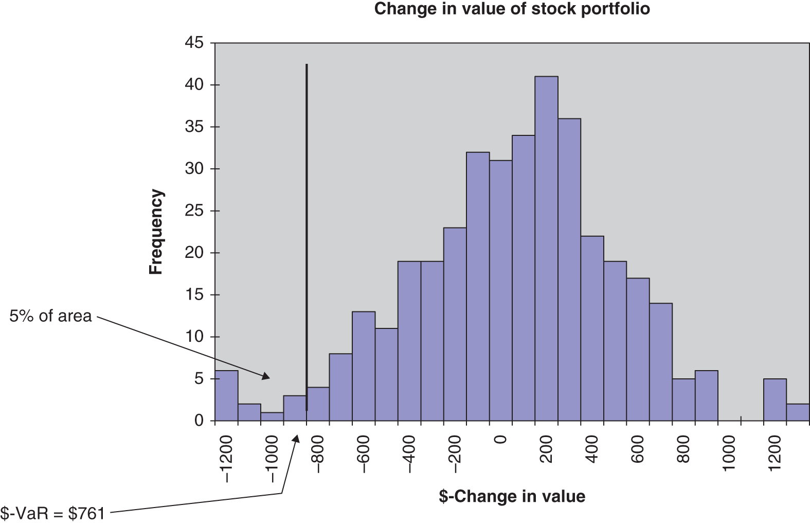
FIGURE 46.2 Historical Simulation
In Figure 46.2 you can clearly see fatter left and right tails, than would be found for the normal distribution. There is also some ‘left skew’ (i.e. more large negative returns than large positive returns). Because we are using an empirical histogram we are not assuming normality. The 5th percentile lower tail cut-off point in Figure 46.2 appears to be around $750. Indeed if we order all the daily changes in value from lowest to highest, the VaR from the historical simulation method at the 5th percentile is found to be $761.
Using the raw historical data on each of the three stock returns, we can calculate the sample standard deviations and correlation coefficients and hence the VaR using the variance-covariance (VCV) method. We find that holding $10,000 in each stock gives a daily![]() as follows:
as follows:
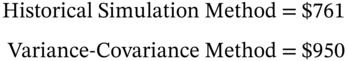
The HS-VaR of $761 is ![]() of the initial value of the portfolio and the VCV-VaR is $950 (3.17% of portfolio value). So there is some difference between the two estimates of VaR which would probably be magnified if we are looking at VaR over a longer horizon than one day.
of the initial value of the portfolio and the VCV-VaR is $950 (3.17% of portfolio value). So there is some difference between the two estimates of VaR which would probably be magnified if we are looking at VaR over a longer horizon than one day.
Why do the two methods, HS and the VCV approach, sometimes give different results? Which is the most accurate? The VCV method assumes that returns are independent (i.e. like a coin flip), that we have accurate forecasts of the standard deviations and correlations, and that all returns are normally distributed. The historical simulation method does not assume normality of stock returns but just takes whatever distribution exists in the historical data. It looks from the histogram in Figure 46.2 that the returns are not normally distributed so we might tend to favour the historical simulation approach. However, we cannot really say which estimate is the more accurate unless we do extensive ‘backtesting’ and compare the forecast errors of competing methods.
The HS method can be used to estimate VaR for any set of assets for which we have a reasonably long series of daily returns and hence daily profits and losses. So in principle the historical data might include the dollar change in value of a portfolio of calls or puts, bonds and foreign assets which can be added to give historical data series for the dollar change in the complete portfolio. There is an added difficulty with coupon paying bonds where calculating price changes may require many different daily changes in spot yields across the whole term structure – this is computationally burdensome.
Accurate estimates of the VaR at the 5th percentile and even more so at the 1st percentile, requires a long time series of data, and this is not always available for some assets. An obvious defect of the HS approach is the complete dependence of the results on the particular data set used. The data set used may contain ‘unusual events’ which are not thought likely to happen again in the immediate future (e.g. sterling leaving the ERM in 1992, the Asian crisis of 1997/8, the events of 9/11 in the USA, the crash of 2008/9, the European debt crisis of 2010). If so, the HS estimate of VaR in the forecast period may not be accurate.
You need quite a lot of data to accurately estimate the 1st percentile VaR from historical data. On the other hand, the longer is our historical data set the more the ‘old’ data may have an influence on our forecast of tomorrow's VaR, as the returns are all given equal weighting. Do we really want the forecast of tomorrow's VaR to be heavily influenced by stock returns that happened say 1,000 days ago (i.e. about 4 years ago when using trading days)?
46.2 BOOTSTRAPPING
A variant of the ‘pure’ historical simulation approach is the bootstrapping technique. As described above, the historical simulation approach consists of ‘one draw’ from the historical data set, where each of the 1,000 daily observations are each chosen once, in order to calculate the portfolio VaR. Suppose we take the view that we only want to use the most recent data to forecast tomorrow's VaR, where ‘recent’ is assumed to be the last 100 days. In other words, we think that historical data from more than 100 days ago is of absolutely no use in forecasting what is likely to happen tomorrow – so we discard it.
It is precisely because tail events are ‘unusual’ that we need quite a lot of data to reliably estimate the VaR. For example, if we are interested in the 1st percentile VaR then in our historical data set, this will only occur 1 in every 100 observations. So, to put an extreme case, suppose you only have 100 observations on daily portfolio returns and 99 of these have a maximum negative value of say 1% but the return on day-1 (i.e. 100 days ago) was minus 8%. Then if you currently hold $100,000 in this portfolio, your forecast of tomorrow's VaR using the HS approach would be ![]() . Given the ‘run’ of actual historical returns do you really believe that $8,000 is a good estimate of what might happen tomorrow? Well only your ‘gut feeling’ can answer this. The figure of $8,000 seems too high a forecast, given the pattern in the historical data. Not only that, but the forecast for 2 days hence would be around
. Given the ‘run’ of actual historical returns do you really believe that $8,000 is a good estimate of what might happen tomorrow? Well only your ‘gut feeling’ can answer this. The figure of $8,000 seems too high a forecast, given the pattern in the historical data. Not only that, but the forecast for 2 days hence would be around ![]() since the ‘–8%’ would drop out of your moving ‘historical window’ of the past 100 days.
since the ‘–8%’ would drop out of your moving ‘historical window’ of the past 100 days.
The dilemma is that you only want to use recent data. But unfortunately that limits the number of observations that are in the 1st percentile of the distribution, from which you are going to make your VaR forecast – in this case a single observation. The bootstrap tries to improve on this by randomly ‘replaying history’ with the fixed sample size of the last 100 days of real data and taking the lowest 1st percentile value for ![]() . We then repeat this a large number of times (say
. We then repeat this a large number of times (say ![]() ) and the best estimate of the VaR is taken to be the average of these 10,000 values of the 1st percentile VaRs.
) and the best estimate of the VaR is taken to be the average of these 10,000 values of the 1st percentile VaRs.
46.2.1 Bootstrap VaR
In the ‘basic bootstrap’ approach the last ![]() portfolio returns (i.e. the values from 901 to 1,000 in the last row of Figure 46.1) are re-sampled with an equal probability of choosing any of the 100 values (using draws from a uniform distribution). We sample with replacement – after each random draw we replace the number chosen in the table – so if we randomly draw the penultimate value +14, we replace it in the table before undertaking the next random draw.
portfolio returns (i.e. the values from 901 to 1,000 in the last row of Figure 46.1) are re-sampled with an equal probability of choosing any of the 100 values (using draws from a uniform distribution). We sample with replacement – after each random draw we replace the number chosen in the table – so if we randomly draw the penultimate value +14, we replace it in the table before undertaking the next random draw.
We can think of each portfolio return for a specific day being numbered from ![]() to 100, corresponding to the last 100 days of historical data. We then draw
to 100, corresponding to the last 100 days of historical data. We then draw ![]() numbers randomly with equal probability. For example, if the 100 random numbers drawn are {92, 70, 10, 87, 55… 92, 27, 70, 54, 10} then we take the change in portfolio value corresponding to these days
numbers randomly with equal probability. For example, if the 100 random numbers drawn are {92, 70, 10, 87, 55… 92, 27, 70, 54, 10} then we take the change in portfolio value corresponding to these days ![]() . Note that some ‘days’ appear more than once (e.g. 92, 70, 10) and others might not appear at all. We then choose the most negative value for the change in portfolio value, from this first random sample of 100 values of
. Note that some ‘days’ appear more than once (e.g. 92, 70, 10) and others might not appear at all. We then choose the most negative value for the change in portfolio value, from this first random sample of 100 values of ![]() . This most negative value is the 1st percentile-VaR for our first ‘random replay of the last 100 days’. For this first bootstrap, assume we obtain
. This most negative value is the 1st percentile-VaR for our first ‘random replay of the last 100 days’. For this first bootstrap, assume we obtain ![]() (loss is reported as a positive number).
(loss is reported as a positive number).
Note that we have allowed any one day's returns to be randomly chosen more than once (or not at all). Although on average you pick any ‘specific day’ just once, because of randomness, some of the 100 days will not be picked at all and some will be picked more than once. We now repeat the above procedure for 1,000 ‘trials/runs/draws’ to obtain 1,000 possible (alternative) values for the 1st percentile-VaR. The results might be:
All the above figures are likely to be losses, since you are always picking the lowest number (i.e. the 1st percentile) from a random sample of ![]() random values. The average of the above 1,000 values might turn out to be
random values. The average of the above 1,000 values might turn out to be ![]() and this is our best forecast of the daily-VaR at the 1st percentile. This ‘Bootstrap VaR’ forecast, done on say Monday, predicts the VaR for Tuesday.
and this is our best forecast of the daily-VaR at the 1st percentile. This ‘Bootstrap VaR’ forecast, done on say Monday, predicts the VaR for Tuesday.
We can also plot the above 1,000 values of ![]() in a histogram and the ‘width’ of this empirical distribution gives you an estimate of the standard deviation around your ‘Bootstrap-VaR’ central estimate:
in a histogram and the ‘width’ of this empirical distribution gives you an estimate of the standard deviation around your ‘Bootstrap-VaR’ central estimate:
where ![]()
You can order the 1,000 values of ![]() from smallest to largest. A 95% confidence interval (i.e. 2.5% in each tail) or ‘range’ for your bootstrap VaR estimate is then the value of the ranked
from smallest to largest. A 95% confidence interval (i.e. 2.5% in each tail) or ‘range’ for your bootstrap VaR estimate is then the value of the ranked ![]() in the 25th position (e.g. $410) and in the 975th position (e.g. $500). Hence your best bootstrap VaR estimate for Tuesday is
in the 25th position (e.g. $410) and in the 975th position (e.g. $500). Hence your best bootstrap VaR estimate for Tuesday is ![]() and the error band is $410 to $500.
and the error band is $410 to $500.
At the end of Tuesday we drop the daily observation on the portfolio return for 100 days ago. We then add one extra day of returns data for the Tuesday, for each stock in our portfolio and recalculate the change in value of the portfolio for the Tuesday. Tuesday's change in portfolio value is now included in the 100 days of data for our bootstrap procedure, which give us the bootstrap VaR forecast for Wednesday. The bootstrap procedure mitigates the ‘lack of data’ problem when calculating the 1st percentile VaR using only ![]() days of actual data and hence in principle we hope to obtain an improved estimate of the portfolio VaR.
days of actual data and hence in principle we hope to obtain an improved estimate of the portfolio VaR.
The bootstrapping technique has similar advantages to the historical simulation approach but still suffers from the problem that the original ![]() historical observations should be ‘representative’ of what might happen in the future. Also the ‘larger simulated’ set of data comes at a price. Since bootstrapping ‘picks out’ each of
historical observations should be ‘representative’ of what might happen in the future. Also the ‘larger simulated’ set of data comes at a price. Since bootstrapping ‘picks out’ each of ![]() daily returns at random (from the 100 historical ‘days’ of data), the simulated returns will ‘lose’ any of the serial correlation which happens to be in the historical returns (i.e. the basic bootstrap method implicitly assumes returns are independent over time). However, even this problem can be tackled by using a ‘block bootstrap’.
daily returns at random (from the 100 historical ‘days’ of data), the simulated returns will ‘lose’ any of the serial correlation which happens to be in the historical returns (i.e. the basic bootstrap method implicitly assumes returns are independent over time). However, even this problem can be tackled by using a ‘block bootstrap’.
46.2.2 Block Bootstrap
To explain the idea behind a block bootstrap, consider the following simple example. Suppose we undertake statistical tests on daily returns and find that serial correlation is positive but only first order (e.g. a moving average error of order one, MA(1)) – so only adjacent returns tend to be correlated. In this case, if we randomly draw the number 92 from the uniform distribution then we would revalue the portfolio not only with the returns on the 92nd day but also on the 91st and 93rd days.
If there is some first order positive serial correlation and the returns on the 92nd day are predominantly negative (positive) then there is a greater than 50% chance that the returns on the two adjacent days are also predominantly negative (positive). We then revalue the portfolio on each of these 3 days. We repeat this random selection in groups of 3 another 30 times to get approximately 100 returns and then choose the most negative value as our first estimate of VaR (at the 1st percentile). We then proceed as before to obtain 10,000 values of the 1st percentile-VaR, and average these 10,000 values, which is our best forecast for the bootstrap-VaR.
Since it is uncertain as to the degree of serial correlation in the data we can undertake a sensitivity analysis by recalculating the BVaR for different ‘block lengths’ (e.g. 3, 5, 12) to see if the estimated BVaR changes dramatically. There are also statistical tests available to choose the most appropriate block lengths.
As regulators allow financial institutions to develop and use their own ‘internal models’ then the HS approach has gained adherents, since although the raw data input requirements are greater than the parametric-VaR approach, the computation is straightforward. Bootstrap-VaR is perhaps done less often because of the need for re-sampling of the original data. These two non-parametric approaches are likely to be more accurate when return distributions are non-normal but in general these two approaches are often treated as complementary rather than as a substitute for the parametric-VCV approach.
46.3 MONTE CARLO SIMULATION
Monte Carlo simulation (MCS) is a very flexible parametric method which allows one to generate the whole distribution of portfolio returns and hence ‘read off’ the VaR at any desired percentile level. In contrast, the HS and bootstrap approaches can only ‘reproduce’ the outcomes that are inherent in the fixed set of historical data. MCS is particularly useful for calculating the VaR for portfolios which contain assets with non-linear payoffs, such as options. It is a parametric method because we assume a specific distribution for the underlying asset returns (e.g. returns on stocks, bonds, long-term interest rates, and spot-FX) and therefore the variances and correlations between these returns need to be estimated, before being used as inputs to the MCS.
However, in MCS one need not assume that the distribution is multivariate normal (although this is often assumed, in practice) and, for example, one could choose to generate the underlying asset returns from a fat-tailed distribution (e.g. Student's t-distribution, mixture normal) or one which has a skewed left tail (e.g. jump diffusion process). However, note that even if the underlying asset returns have a multivariate normal distribution, the distribution of the change in value of a portfolio of options will not be multivariate normal, because of the non-linear relationship between the underlying asset return and option premia – as in the Black–Scholes formula.
Within the MCS framework applied to options we can also choose whether to calculate the change in value of the portfolio of options by using the full valuation method (e.g. Black–Scholes formula), or using only the ‘delta’ or the ‘delta+gamma’ approximation or indeed, other methods of calculating option premia (e.g. assuming stochastic volatility). Of course, measuring VaR using the linear/delta method or the ‘delta+gamma’ approximation may not be accurate for options that are ‘near-the-money’, because these have a very pronounced non-linear response to changes in the underlying asset price.
We begin by showing how to measure the VaR of a single option using MCS and then move on to consider the VaR for portfolios which contains several options.
46.3.1 Single Asset: Long Call
Suppose you hold a long call on a stock with ![]() ,
, ![]() ,
, ![]() ,
, ![]() and with
and with ![]() year to maturity and the initial value of the call using Black–Scholes is
year to maturity and the initial value of the call using Black–Scholes is ![]() . What is the VaR of this call over a 30-day horizon? We simulate the stock price over 30 days assuming it follows a geometric Brownian motion (GBM) with the ‘real world’ mean return on the stock
. What is the VaR of this call over a 30-day horizon? We simulate the stock price over 30 days assuming it follows a geometric Brownian motion (GBM) with the ‘real world’ mean return on the stock ![]() .
.
After 30 days, the simulated stock price is ![]() and the ‘new’ call premium is given by the Black–Scholes equation
and the ‘new’ call premium is given by the Black–Scholes equation ![]() , where we have assumed that the other inputs
, where we have assumed that the other inputs ![]() and
and ![]() remain constant over the 30-day horizon. The dollar change in value for this first ‘run’ of the MCS is
remain constant over the 30-day horizon. The dollar change in value for this first ‘run’ of the MCS is ![]() . We now repeat the above for say
. We now repeat the above for say ![]() runs and obtain
runs and obtain ![]() (for
(for ![]() ). Finally we order the values of
). Finally we order the values of ![]() from lowest to highest or plot them in a histogram (Figure 46.3). The 5th (1st) percentile lower cut of point gives the VaR, which here is $14.5 ($17.9), that is about 57% (70%) of the initial call premium
from lowest to highest or plot them in a histogram (Figure 46.3). The 5th (1st) percentile lower cut of point gives the VaR, which here is $14.5 ($17.9), that is about 57% (70%) of the initial call premium ![]() .
.
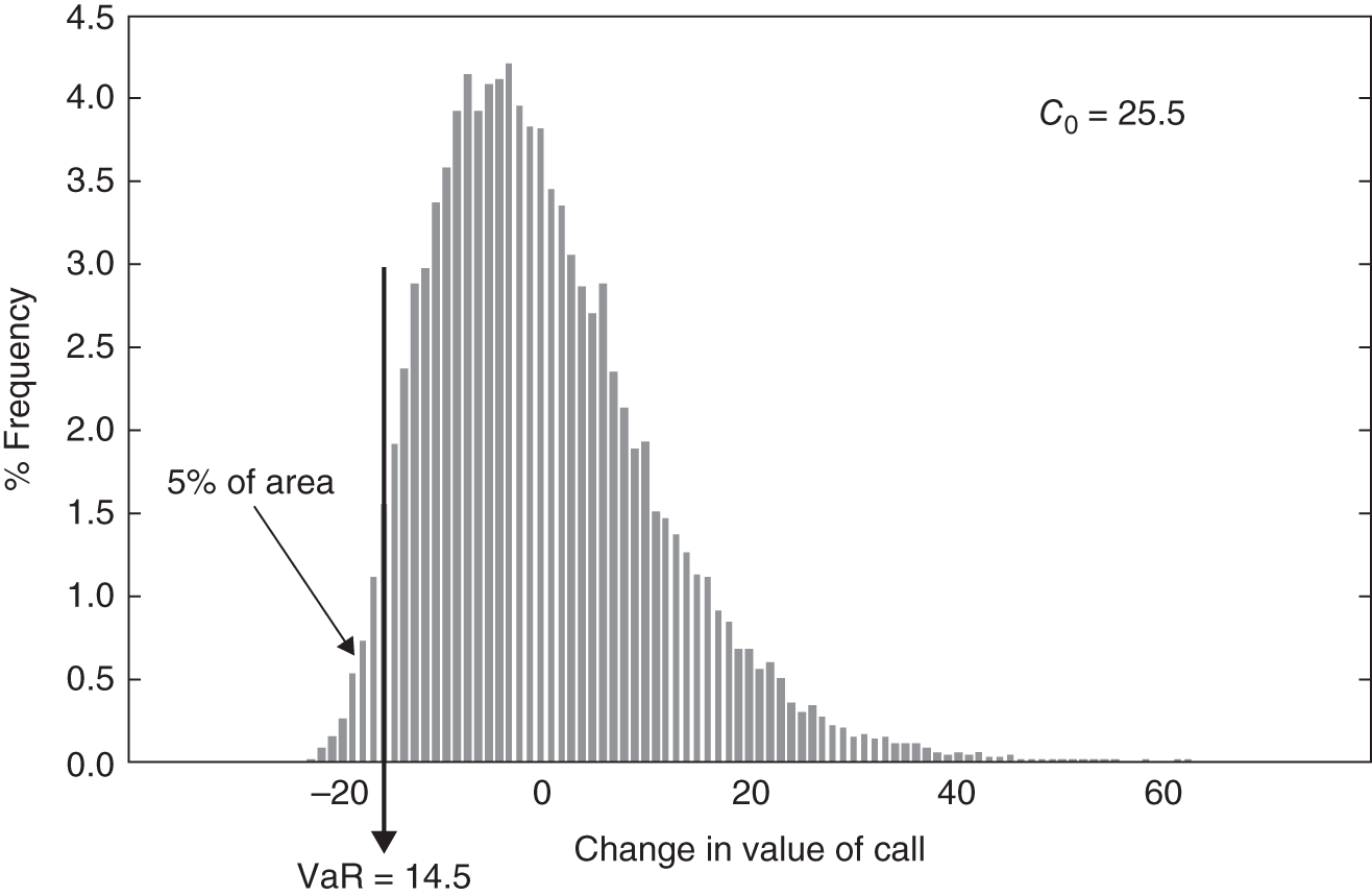
FIGURE 46.3 VaR of one long call option
Even though stock returns are assumed to be normally distributed, the histogram of the call premium (Figure 46.3) is non-normal because of the curvature of the relationship between the call premium and the stock price. We valued the option using a closed-form solution (Black–Scholes) which is a ‘full valuation method’. We could instead have approximated the change in the option premium using either the linear ‘delta approximation’ or the ‘delta+gamma’ approximation. The choice here depends on the degree of accuracy versus the tractability of a particular valuation approach. We discuss this further below.
46.3.2 Options on Different Stocks
To make the algebra simple, assume we hold ![]() options (calls or puts) with option premiums
options (calls or puts) with option premiums ![]() on the same underlying stock (Exxon Mobile) with stock price
on the same underlying stock (Exxon Mobile) with stock price ![]() and
and ![]() options with option premium
options with option premium ![]() on a different underlying stock (AT&T) with stock price
on a different underlying stock (AT&T) with stock price ![]() .
.
Both stocks are ‘domestic’ (e.g. US stocks). If ![]() then the options are held long (short). The Monte Carlo methodology to calculate the 30-day VaR at the 5th percentile, over a 30-day horizon, involves the following steps.
then the options are held long (short). The Monte Carlo methodology to calculate the 30-day VaR at the 5th percentile, over a 30-day horizon, involves the following steps.
- The initial value of the option's portfolio is:
(46.1)
Assume we value the options using the Black–Scholes formula. The initial two option premia (
 ) are
) are 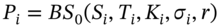 where
where  is the strike price,
 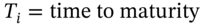 ,
,  is the annual stock return volatility and
  is the risk-free rate. We assume the volatility and interest rate remain constant over the 30-day horizon.
 - Using statistical estimates of volatilities and correlations the following recursive equations:
(46.2a)are used to generate the two stock price series over 30 trading days,3 where

 . This is the MCS. Each of the
  but
but  and
and  are contemporaneously correlated with a correlation coefficient of
  . This means the simulations mimic the correlation between the two stock returns found in the actual real world data. (The
  are generated using the Choleski decomposition outlined in Chapter 26.)
 - New Black–Scholes values for options prices and the portfolio value at
 are:
are:
 (46.3)
Hence the first run of the MCS
 , the change in value of the options portfolio is:(46.4)
We repeat steps 2 and 3, ![]() times and obtain 10,000 simulated values for the 30-day change in the $-value of the options portfolio
times and obtain 10,000 simulated values for the 30-day change in the $-value of the options portfolio ![]() . We then locate the 5th percentile in the left tail of the distribution – this is the portfolio-VaR over 30 days.
. We then locate the 5th percentile in the left tail of the distribution – this is the portfolio-VaR over 30 days.
46.3.3 Approximations: Delta and ‘Delta+Gamma’
Above, we used the Black–Scholes equation to price the option – known as the ‘full valuation method’. Alternatively, one can approximate the change in price of an option using the option's delta ![]() (evaluated at the initial stock price at t = 0). Consider estimating the VaR over 30 days for one long call, using (i) the full valuation method (Black–Scholes), (ii) the delta approximation, and (iii) the ‘delta plus gamma’ approximation. Using the delta approximation:
(evaluated at the initial stock price at t = 0). Consider estimating the VaR over 30 days for one long call, using (i) the full valuation method (Black–Scholes), (ii) the delta approximation, and (iii) the ‘delta plus gamma’ approximation. Using the delta approximation:
where ![]() is the simulated value of the stock price at
is the simulated value of the stock price at ![]() . Using
. Using ![]() provides a (linear) first order approximation to the change in the call premium. The second-order approximation including the option's gamma is:
provides a (linear) first order approximation to the change in the call premium. The second-order approximation including the option's gamma is:
A comparison of VaR outcomes is given in Table 46.1. At the 1st percentile, the full valuation method gives a VaR of $17.9 (a fall of 30% of the initial call premium of $25.5) while the delta approximation gives $21.1 (a fall of 17%), which implies a substantial error. The ‘delta+gamma’ method gives $17.8 (a fall of 30% of the initial call premium) which is very close to that for the full valuation method using Black–Scholes.
TABLE 46.1 Delta and delta+gamma approximation
| Input | |||
|
|
|
||
| Value at risk | |||
| Percentile | Full valuation (BS) | Delta approximation | Delta and gamma |
| 1st | $ 17.9 (70.4%) | $ 21.1 (82.7%) | $ 17.8 (69.9%) |
| 5th | $ 14.5 (57.0%) | $ 15.7 (61.8%) | $ 13.9 (54.7%) |
Notes: Figures in parentheses are the percentage of initial in value (i.e. $VaR/Initial call premium).
If we have a portfolio of options (on the same underlying stock-i), the delta and gamma in the above formula are the ‘portfolio-delta’ and ‘portfolio-gamma’ and the dollar change in value is:
For a portfolio of options on different stocks (e.g. options on AT&T, options on Exxon, etc.), the change in value for each option on stock-i is given in Equation (46.7) and the change in total portfolio value (i.e. containing all the options) of the n-different options is  . In the MCS, the stock prices are simulated as in Equation (46.2) incorporating all the correlations between the n underlying stock returns, using the (n × n) Choleski decomposition.
The delta+gamma approximation can be used when the options being considered have no closed-form solution but we are able to get estimates of delta and gamma from numerical approaches to pricing the option (such as MCS or the BOPM).
In the above Monte Carlo simulation we assume normality of (log) stock returns. But if stock return distributions in reality have fat tails (or are left skewed) then the estimated VaR is likely to be an underestimate of the true VaR. We then need to use MCS, but perform sampling from return distributions that are more representative of the actual empirical data (e.g. Student's t-distribution which is symmetric but with fatter tails than the normal distribution).
46.4 ALTERNATIVE METHODS
VaR is an attempt to encapsulate in a single figure, the dollar-risk of a portfolio of assets, over a specific horizon with a given probability. The VaR can be calculated in a number of different ways. For example, the variance-covariance (VCV) parametric approach assumes (multivariate) normally distributed returns and uses specific forecasts of volatilities and correlations (e.g. EWMA). When the portfolio contains options then the ‘parametric’ Monte Carlo method is often used.
Clearly these approaches are subject to ‘model error’, since the estimated variances and covariances may be incorrect. In contrast, in the ‘non-parametric’ historical simulation method and bootstrapping we observe how our current portfolio value would have changed, given the actual historical data on returns. Non-parametric methods require a substantial amount of data and the results can sometimes be highly dependent on the sample of historical data chosen.
Let us examine some of the problems of the above approaches which are all based on forecasts derived from ‘averaging’ over a sample of recent data. For example, in the VCV approach a portfolio with market value ![]() and
and ![]() (per day) has a VaR of $10m over 1 day at the 5th percentile
(per day) has a VaR of $10m over 1 day at the 5th percentile ![]() . This indicates that for about 19 days out of 20, losses should not exceed $10m and losses could exceed $10m in about 1 day out of every 20. However the VaR figure gives no indication of what the actual losses on any specific day will be. If returns are (conditionally) normal then the cut off point for the 0.5% left-tail is 3.2
. This indicates that for about 19 days out of 20, losses should not exceed $10m and losses could exceed $10m in about 1 day out of every 20. However the VaR figure gives no indication of what the actual losses on any specific day will be. If returns are (conditionally) normal then the cut off point for the 0.5% left-tail is 3.2 ![]() , giving a VaR of $19.4m. So we can be ‘pretty sure’ losses will not exceed $20m – in fact, we expect to lose more than $20m, only 5 days in every 1,000 days. But even then, we cannot be absolutely sure of the actual dollar loss because:
, giving a VaR of $19.4m. So we can be ‘pretty sure’ losses will not exceed $20m – in fact, we expect to lose more than $20m, only 5 days in every 1,000 days. But even then, we cannot be absolutely sure of the actual dollar loss because:
- Even with the normal distribution, there is a small probability of a very large loss.
- Actual returns may have fatter tails than those of the normal distribution, so larger, more frequent dollar losses (on average) will occur (relative to those assuming normality).
- Correlations and volatilities can change very sharply. For example, within a 3-month period the daily correlation between daily returns on the Nikkei 225 and the FTSE 100 have varied from +0.9 to –0.9 and the daily volatility on the Nikkei 225 in a specific 3-month period varied between 0.7% to 1.8% per day.
All of the methods discussed (e.g. the VCV parametric approach, historical simulation, Monte Carlo simulation) generally assume the portfolio is held fixed over the holding period considered. This limitation becomes more unrealistic the longer the time horizon over which VaR is calculated. For example, while one may not be able to easily liquidate a position within a day (particularly in crisis periods), this is not necessarily true over periods longer than say 10 days.
Another crucial dimension which is missing in all the approaches, is the ‘bounce-back period’. On a mark-to-market basis, estimated cumulative 10-day losses might be large but if markets fully recover over the next 20 days, the cumulative actual losses over 30 days could be near zero. It may therefore be worthwhile to examine the VaR without using the ![]() scaling factor, but instead trying to get an explicit estimate of volatilities over longer horizons (e.g. where returns might exhibit more mean reversion). However, it requires a substantial amount of data to accurately model and forecast volatilities over longer horizons.
scaling factor, but instead trying to get an explicit estimate of volatilities over longer horizons (e.g. where returns might exhibit more mean reversion). However, it requires a substantial amount of data to accurately model and forecast volatilities over longer horizons.
46.4.1 Stress Testing
So far our VaR calculations, whether using the VCV approach or historical simulation/bootstrapping approaches, have their difficulties – the former assumes normally distributed returns and the latter require a relatively long run of past data. Both approaches assume that an average of recent past data is a good guide to what might happen in the future. Because of this dependence on a particular data set, they are often supplemented by stress tests. Stress testing estimates the sensitivity of a portfolio to specific ‘extreme movements’ in certain key returns. It tells you how much you will lose in a particular state of the world but usually gives no indication of how likely it is that this state of the world will actually occur.
Choice of ‘extreme movements’ may be based on particular crisis periods (e.g. 1987 stock market crash, the 1992 ‘crisis’ when sterling left the ERM, the 1997–8 Russian bond default, the Asian currency crisis of 1997/8, the banking crisis of 2008–10, the Greek sovereign debt crisis of 2010–13). It follows that the implicit volatilities and correlations between asset returns are specific to the historical crisis periods chosen for the stress tests – and these are likely to be periods when correlations tend to increase dramatically.
Alternatively, the financial institution can simply revalue its existing portfolio using whatever returns it thinks ‘reasonable and informative’ – the danger here is outcomes which bear little or no relation to actual historical events or which mimic events which have never occurred and are unlikely to occur in the future – so there is a lot of judgement required when undertaking a ‘reasonable’ scenario.
Clearly, this type of stress testing is best done for relatively simple portfolios since otherwise the implicit correlations for the chosen scenario may be widely at variance with those in the historical data or even for any conceivable future event. But note another danger of stress testing – namely, that a portfolio might actually benefit from ‘extreme’ movements yet be vulnerable to ‘small’ movements. For example, the ‘U’ shaped payoff for a long straddle (buy a call and a put with the same strike and expiration date), indicates large profits if the underlying price moves by a large amount in either direction (prior to or at maturity) – but a loss of some of the option premia, if the underlying price moves by only a small amount.
In general, stress testing has several limitations and the same stress-testing scenario is unlikely to be informative for all institutions (portfolios). The choice of inputs for the stress test(s) will depend on the financial institution's or regulator's assessment of the likely source of the key ‘prices’ and sensitivities to changes in these prices, given its portfolio composition. For example, a commodities dealer is unlikely to find a stress test of a parallel shift in interest rates of 200 bps useful but would base her stress tests on movements in spot and derivatives prices of major commodities. One can also usefully turn the scenario approach ‘on its head’ and ask ‘Given my portfolio, what set of plausible scenarios (for stock prices, interest rates, exchange rates, etc.) will yield very bad outcomes?’
Stress testing is therefore a useful complement to the usual VaR calculations but requires considerable judgement in its practical implementation. Because of the perceived failure of risk management techniques like VaR in the 2008–9 financial crisis, regulators have placed additional emphasis on stress testing, particularly for ‘systemically important’ banks.
46.4.2 Extreme Value Theory
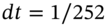
Another method for calculating VaR which concentrates on the tails of the distribution is extreme value theory (EVT). This method is used in the natural sciences for estimating the expected maximum extreme ‘loss’, with a specific degree of confidence, over a given horizon (e.g. expected losses, at a given confidence level, from the failure of a dam or nuclear power plant within the next 5 years). In a very broad sense, the EVT approach is a mixture of the historical simulation approach together with the estimation of a smooth curve to represent the ‘true’ shape of the tail of the distribution. EVT uses only data in the extreme tail of losses and discards the rest of the data, namely small losses and all gains – as the latter data is assumed to be uninformative in forecasting extreme losses that might happen in the future.
Suppose we have data on actual daily changes in the value of a stock portfolio over the last 500 days. With EVT we have to choose where the tail of ‘extreme losses’ begins. Suppose we assume ‘extreme losses’ are those below the 5th percentile (left-tail) and this gives us 25 values for losses that are larger than ![]() , say.4 If we plot a histogram of these worst outcomes it would probably look very ‘lumpy’ (Figure 46.4).
, say.4 If we plot a histogram of these worst outcomes it would probably look very ‘lumpy’ (Figure 46.4).
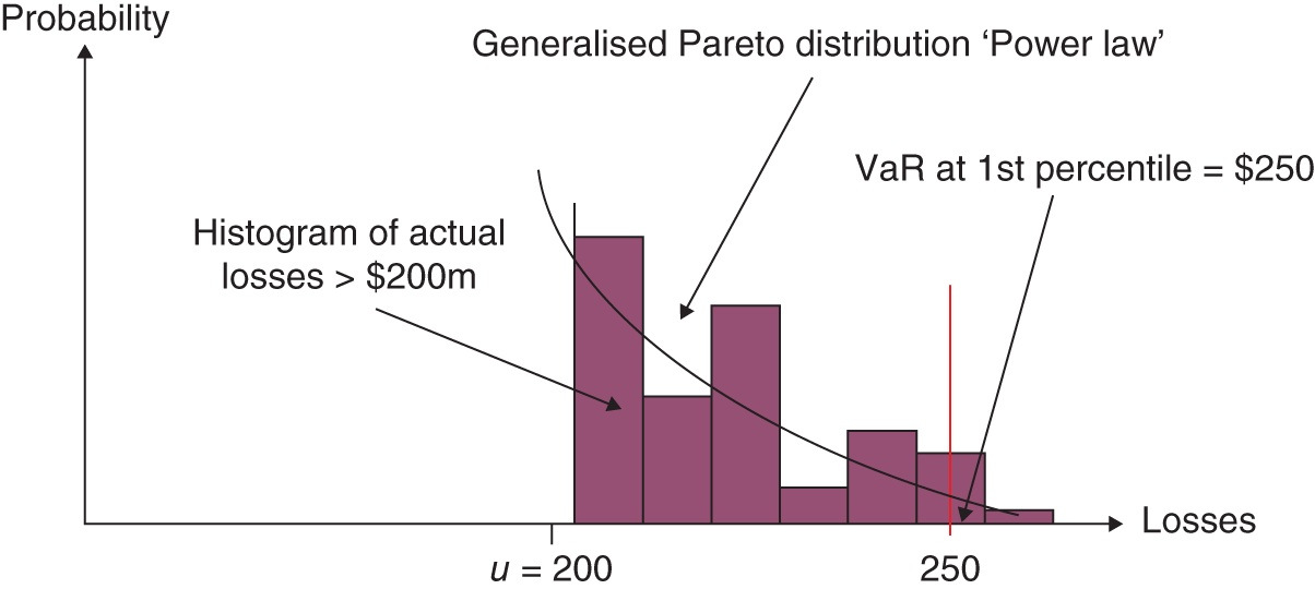
FIGURE 46.4 EVT
What EVT does is to fit a ‘smooth curve’ through this histogram of extreme values, without imposing any specific assumptions concerning the rest of the distribution. Having estimated the smooth curve, you can then ‘read off’ the VaR at any percentile in the tail (e.g. VaR at the 1st percentile as in Figure 46.4). There is an art in getting EVT to estimate the ‘true’ distribution for tail losses since the position and shape of the tail depends on how many of our empirical data points we choose to include as ‘extreme’.
Danielsson and de Vries (1997) report that for VaRs below 5th percentile, the VCV approach tends to underpredict the occurrence of tail events, the historical simulation approach tends to overpredict, while the EVT approach performs well. Hence the EVT approach may provide a more accurate VaR estimate, the ‘smaller’ the percentile of the distribution one is interested in.
46.5 SUMMARY
- The variance-covariance (VCV) method of forecasting daily, weekly or monthly VaR assumes all asset returns in a portfolio are
 – this is a reasonable assumption for a portfolio of domestic stocks, foreign stocks and futures contracts, a workable assumption for bonds, FRNs and swaps but is not accurate for portfolios containing options.
 - The historical simulation method is reasonably accurate in predicting VaR between the 1st and 5th percentiles but it requires a substantial amount of data and is a little inflexible (e.g. it is difficult to do sensitivity analysis), compared with the standard parametric VCV method.
- The bootstrap approach allows a non-parametric calculation of VaR using only recent historical data – but it still relies on past data being representative of what might happen in the near future.
- VaR for portfolios containing ‘plain vanilla’ European options can be estimated using Monte Carlo simulation (MCS).
- The extreme value theory (EVT) approach uses data only from the extreme tail of the empirical loss distribution and estimates a smooth curve for the observed extreme losses, from which we can then obtain the VaR at any desired (low) percentile. EVT is more complex than other parametric methods and (like them) is subject to estimation error.
- Stress testing provides a complementary approach to measuring market risk to that provided by other methods such as VCV, EVT, MCS, HS, and bootstrapping. Much judgement is required when undertaking alternative scenarios and the probability of various outcomes (usually) cannot be assessed.
- Alternative approaches used in calculating VaR for large diverse international portfolios of stocks, bonds, swaps, futures, and options contracts are impressive. However, a large element of judgement and common sense is required when using and interpreting results from any of these approaches.
EXERCISES
Question 1
Briefly explain the difference between Monte Carlo simulation (MCS) and stress testing in assessing the riskiness of a portfolio of assets.
Question 2
In a Monte Carlo simulation indicate the steps involved in calculating the VaR over a 10-day horizon, for a long call option on a stock (assuming Black–Scholes holds). For expositional purposes assume ![]() ,
, ![]() ,
, ![]() ,
, ![]() ,
, ![]() (year) and the mean return on the stock is
(year) and the mean return on the stock is ![]() p.a.
p.a.
Question 3
How would you use asset returns over the last 1,000 days to obtain the daily VaR at the 5th percentile, using historical simulation?
Question 4
Name two possible weaknesses when using historical simulation to obtain the daily VaR (at the 5th percentile) from returns over the last 1,000 days.
Question 5
A US investor is short $10m in each of stock-1 and stock-2 and long $10m in stock-3. The returns over the last 5-days on these three stocks are:
| Days = | 1 | 2 | 3 | 4 | 5 |
| % Return-1 | 3 | −2 | 8 | −5 | −1 |
| % Return-2 | 2 | 1 | 3 | 4 | 3 |
| % Return-3 | −4 | −5 | −5 | −2 | −1 |
A US investor decides to use the historical simulation method with only the last 5 days of data to forecast her VaR for day-6, at the 20th percentile. What is the VaR?
Question 6
If daily stock returns are autocorrelated (with a first order autocorrelation coefficient of +0.2) how might this feature of the data be incorporated in a MCS?
Question 7
Does the (standard) historical simulation method incorporate the volatility and correlations between the assets that make up the portfolio, when estimating the portfolio VaR?
Question 8
When using MCS (and Brownian motion) to obtain the VaR of a portfolio of options on different underlying stocks, what key assumptions do you make?
Question 9
You hold one long European put (on 100 stocks of XYZ) and 50 stocks of ABC. Explain how you can use Monte Carlo simulation to obtain the 10-day VaR of this portfolio (at the 1st percentile)?
NOTES
- 1 In the variance-covariance method we would usually scale up daily stock return volatility using the root-T rule – but this requires that stock returns are independent over time (and identically distributed). The basic HS method also requires stock returns to be independent over time.
- 2 This ordering ignores any autocorrelation in returns and essentially assumes independence of portfolio returns over time.
- 3 This equation gives an exact lognormal distribution for S for any size of step
 . Because of this we do not have to use the recursion over 30 separate days (with 30 separate draws of the
  ) we can obtain
  in ‘one-step’ using only one draw of
  and using
  where
where  . This speeds up the calculation of
  compared with the 30-day recursion, where we use ‘30 draws’ of
  .
. - 4 The choice of
 is a trade off between having data which we believe is truly in the left tail and having enough data points in the ‘extreme tail’ (of the histogram) to obtain a reasonable estimate for a smooth curve to represent the shape and position of the tail of the distribution.