26. Cuttings

Search in book...
Toggle Font Controls
Create new playlist

Name your new playlist

Playlist description (optional)
Sign In

Email address

Password

Forgot Password?

or

Continue with Facebook

Continue with Google
Sign Up

Full Name

Email address

Confirm Email Address

Password

or

Continue with Facebook

Continue with Google

Bernard Chazelle

Princeton University

26.1Introduction

26.2The Cutting Construction

Geometric Sampling•Optimal Cuttings

26.3Applications

Point Location•Hopcroft’s Problem•Convex Hulls and Voronoi Diagrams•Range Searching

Acknowledgments

References

26.1Introduction

For divide-and-conquer purposes, it is often desirable to organize a set S of n numbers into a sorted list, or perhaps to partition it into two equal-sized groups with no element in one group exceeding any element in the other one. More generally, we might wish to break up S into k groups of size roughly n/k, with again a total ordering among the distinct groups. In the first case we sort; in the second one we compute the median; in the third one we compute quantiles. This is all well known and classical. Is it possible to generalize these ideas to higher dimension? Surprisingly the answer is yes. A geometric construction, known as an ɛ-cutting, provides a space partitioning technique that extends the classical notion of selection to any finite dimension. It is a powerful, versatile data structure with countless applications in computational geometry.

Let H be a set n hyperplanes in Rd. Our goal is to divide up Rd into simplices, none of which is cut by too many of the n hyperplanes. By necessity, of course, some of the simplices need to be unbounded. We choose a parameter ɛ > 0 to specify the coarseness of the subdivision. A set $C$ $C$ of closed full-dimensional simplices is called an ɛ-cutting for H (Figure 26.1) if:

1.The union of the simplices is Rd, and their interiors are mutually disjoint;

2.The interior of any simplex is intersected by at most ɛn hyperplanes of H.

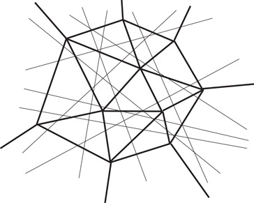
Figure 26.1A two-dimensional cutting.

Historically, the idea of using sparsely intersected simplices for divide and conquer goes back to Clarkson [1] and Haussler and Welzl [2], among others. The definition of an ɛ-cutting given above is essentially due to Matoušek [3]. Efficient but suboptimal constructions were given by Agarwal [4,5] for the two-dimensional case and Matoušek [3,6,7] for arbitrary dimension. The optimal ɛ-cutting construction cited in the theorem below, due to Chazelle [8], is a simplification of an earlier design by Chazelle and Friedman [9].

Theorem 26.1

Given a set H of n hyperplanes in Rd, for any 0 < ɛ < 1, there exists an ɛ-cutting for H of size O(ɛ^−d), which is optimal. The cutting, together with the list of hyperplanes intersecting the interior of each simplex, can be found deterministically in O(nɛ^1−d) time.

26.2The Cutting Construction

This section explains the main ideas behind the proof of Theorem 26.1. We begin with a quick overview of geometric sampling theory. For a comprehensive treatment of the subject, see References 10 and 11.

26.2.1Geometric Sampling

A set system is a pair $Σ = (X, R)$ $Σ = (X, R)$ , where X is a set and $R$ $R$ is a collection of subsets of X. In our applications, X ⊂ Rd and each $R \in R$ $R \in R$ is of the form X ∩ f(K), where K is a fixed region of Rd and f is any member of a fixed group F of transformations. For example, we might consider n points in the plane, together with the subsets lying inside any triangle congruent to a fixed triangle.

Given Y ⊆ X, we define the set system “induced by Y” to be $(Y, R |_{Y})$ $(Y, R |_{Y})$ , with $R |_{Y} = {Y \cap R | R \in R}$ $R |_{Y} = {Y \cap R | R \in R}$ . The VC-dimension (named for Vapnik and Chervonenkis [12]) of Σ is defined as the maximum size of any Y such that $R |_{Y} = 2^{Y}$ $R |_{Y} = 2^{Y}$ . For example, the VC-dimension of the infinite geometric set system formed by points in the plane and halfplanes is 3. The shatter function $π_{R} (m)$ $π_{R} (m)$ of the set system $Σ = (X, R)$ $Σ = (X, R)$ is the maximum number of subsets in the set system $(Y, R |_{Y})$ $(Y, R |_{Y})$ induced by any Y ⊆ X of size m. If $π_{R} (m)$ $π_{R} (m)$ is bounded by cmd, for some constants c, d > 0, then the set system is said to have a shatter function exponent of at most d. It was shown in References 12–14 that, if the shatter function exponent is O(1), then so is the VC-dimension. Conversely, if the VC-dimension is d ≥ 1 then, for any m ≥ d, $π_{R (m)} < (e m / d)^{d}$ $π_{R (m)} < (e m / d)^{d}$ .

We now introduce two fundamental notions: ɛ-nets and ɛ-approximations. For any 0 < ɛ < 1, a set N ⊆ X is called an ɛ-net for a finite set system $(X, R)$ $(X, R)$ if N ∩ R ≠ for any $R \in R$ $R \in R$ with |R|/|X| > ɛ. A finer (but more costly) sampling mechanism is provided by an ɛ-approximation for $(X, R)$ $(X, R)$ , which is a set A ⊆ X such that, given any $R \in R$ $R \in R$ ,

| \frac{| R |}{| X |} - \frac{| A \cap R |}{| A |} | \leq ε .

$| \frac{| R |}{| X |} - \frac{| A \cap R |}{| A |} | \leq ε .$

Some simple structural facts about nets and approximations:

Lemma 26.1

If X1, X2 are disjoint subsets of X of the same size, and A1, A2 are same-size ɛ-approximations for the subsystems induced by X1, X2 (respectively), then A1 ∪ A2 is an ɛ-approximation for the subsystem induced by X1 ∪ X2.

Lemma 26.2

If A is an ɛ-approximation for $(X, R)$ $(X, R)$ , then any ɛ′-approximation (resp. -net) for $(A, R |_{A})$ $(A, R |_{A})$ is also an (ɛ + ɛ′)-approximation (resp. -net) for $(X, R)$ $(X, R)$ .

In the absence of any restrictive assumption on the set system, it is natural to expect the sample size to depend on both the desired accuracy and the size of the set system itself.

Theorem 26.2

Given a set system $(X, R)$ $(X, R)$ , where |X| = n and $| R | = m$ $| R | = m$ , for any 1/n ≤ ɛ < 1, it is possible to find, in time O(nm), an ɛ-net for $(X, R)$ $(X, R)$ of size O(ɛ⁻¹ log m) and an ɛ-approximation for $(X, R)$ $(X, R)$ of size O(ɛ⁻² log m).

If we assume bounded VC-dimension, everything changes. In fact the key result in geometric sampling theory is that, for any given level of accuracy, the sample size need not depend on the size of the set system.

In practice, geometric set systems often are “accessible” via an oracle function that takes any Y ⊆ X as input and returns the list of sets in $R |_{Y}$ $R |_{Y}$ (each set represented explicitly). We assume that the time to do that is O(|Y|^d+1), which is linear in the maximum possible size of the oracle’s output, where d is the shatter function exponent. For example, in the case of points and disks in the plane, we have d = 3, and so this assumes that, given n points, we can enumerate all subsets enclosed by a disk in time O(n4). To do this, enumerate all k-tuples of points (k ≤ 3) and, for each tuple, find which points lie inside the smallest disk enclosing the k points. The main result below is stated in terms of the shatter function exponent d, but the same results hold if d denotes the VC-dimension.

Theorem 26.3

Given a set system $(X, R)$ $(X, R)$ of shatter function exponent d, for any ɛ ≤ 1/2, an ɛ-approximation for $(X, R)$ $(X, R)$ of size O(dɛ⁻² log dɛ⁻¹) and an ɛ-net for $(X, R)$ $(X, R)$ of size O(dɛ⁻¹ log dɛ⁻¹) can be computed in time O(d)^3d(ɛ⁻² log dɛ⁻¹)d|X|.

Vapnik and Chervonenkis [12] described a probabilistic construction of ɛ-approximations in bounded VC-dimension. The deterministic construction stated above is due to Chazelle and Matoušek [15], and builds on earlier work [3,6,7,9]. Haussler and Welzl [2] proved the upper bound on the size of ɛ-nets. The running time for computing an ɛ-net was improved to O(d)^3d(ɛ⁻¹ log dɛ⁻¹)d|X| by Brönnimann, Chazelle, and Matoušek [16], using the concept of a sensitive ɛ-approximation. Komlós, Pach, and Woeginger [17] showed that, for any fixed d, the bound of O(ɛ⁻¹ log ɛ⁻¹) for ɛ-nets is optimal in the worst case (see also Reference 18). The situation is different with ɛ-approximations: if d > 1 is the VC dimension, then there exists an ɛ-approximation for $(X, R)$ $(X, R)$ of size O(ɛ^−2+2/(d+1)) [19,20].

An important application of ɛ-approximations is for estimating how many vertices in an arrangement of hyperplanes in Rd lie within a given convex region. Let $Σ = (H, R)$ $Σ = (H, R)$ be the set system formed by a set H of hyperplanes in Rd, where each $R \in R$ $R \in R$ is the subset of H intersected by an arbitrary line segment. Let σ be a convex body (not necessarily full-dimensional). In the arrangement formed by H within the affine span of σ, let V (H, σ) be the set of vertices that lie inside σ. The following was proven in References 8 and 16.

Theorem 26.4

Given a set H of hyperplanes in Rd in general position, let A be an ɛ-approximation for $Σ = (H, R)$ $Σ = (H, R)$ . Given any convex body σ of dimension k ≤ d,

| \frac{| V (H, σ) |}{| H |^{k}} - \frac{| V (A, σ) |}{| A |^{k}} | \leq ε .

$| \frac{| V (H, σ) |}{| H |^{k}} - \frac{| V (A, σ) |}{| A |^{k}} | \leq ε .$

26.2.2Optimal Cuttings

For convenience of exposition, we may assume that the set H of n hyperplanes in Rd is in general position. Let $A (H)$ $A (H)$ denote the arrangement formed by H. Obviously, no simplex of an ɛ-cutting can enclose more than O(ɛn)d vertices. Since $A (H)$ $A (H)$ itself has exactly $(\begin{matrix} n \\ d \end{matrix})$ $(\begin{matrix} n \\ d \end{matrix})$ vertices, we should expect to need at least on the order of ɛ^−d simplices. But this is precisely the upper bound claimed in Theorem 26.1, which therefore is asymptotically tight.

Our starting point is an ɛ-net N for H, where the underlying set system $(X, R)$ $(X, R)$ is formed by a set X of hyperplanes and the collection $R$ $R$ of subsets obtained by intersecting X with all possible open d-simplices. Its VC-dimension is bounded, and so by Theorem 26.3 an ɛ-net N of size O(ɛ⁻¹ log ɛ⁻¹) can be found in nɛ^−O(1) time.

We need to use a systematic way to triangulate the arrangement formed by the ɛ-net. We build a canonical triangulation of $A (N)$ $A (N)$ by induction on the dimension d (Figure 26.2). The case d = 1 is trivial, so we assume that d > 1.

1.Rank the vertices of $A (N)$ $A (N)$ by the lexicographic order of their coordinate sequences.

2.By induction, form a canonical triangulation of the (d − 1)-dimensional arrangement made by each hyperplane with respect to the n − 1 others.

3.For each cell (i.e., full-dimensional face) σ of $A (N)$ $A (N)$ , lift toward its lowest-ranked vertex v each k-simplex (k = 0,…, d − 2) on the triangulated boundary of σ that does not lie in a (d − 1)-face of $A (N)$ $A (N)$ that is incident to v.

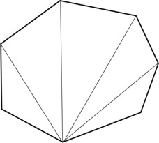
Figure 26.2A canonical triangulation.

It is not hard to see that the combinatorial complexity (i.e., number of all faces of all dimensions) of the canonical triangulation of $A (N)$ $A (N)$ is asymptotically the same as that of $A (N)$ $A (N)$ , which is O(ɛ⁻¹ log ɛ⁻¹)d. Therefore, the closures of its cells constitute an ɛ-cutting for H of size O(ɛ⁻¹ log ɛ⁻¹)d, which is good but not perfect. For optimality we must remove the log factor.

Assume that we have at our disposal an optimal method for building an ɛ0-cutting of size $O (ε_{0}^{- d})$ $O (ε_{0}^{- d})$ , for some suitably small constant ɛ0. To bootstrap this into an optimal ɛ-cutting construction for any ɛ, we might proceed as follows: Beginning with a constant-size cutting, we progressively refine it by producing several generations of finer and finer cuttings, $C_{1}, C_{2}$ $C_{1}, C_{2}$ , etc, where $C_{k}$ $C_{k}$ is an $ε_{0}^{k}$ $ε_{0}^{k}$ -cutting for H of size O(ɛ^−dk). Specifically, assume that we have recursively computed the cutting $C_{k}$ $C_{k}$ for H. For each $σ \in C_{k}$ $σ \in C_{k}$ , we have the incidence list H_σ of the hyperplanes intersecting the interior of σ. To compute the next-generation cutting $C_{k + 1}$ $C_{k + 1}$ , consider refining each σ in turn as follows:

1.Construct an ɛ0-cutting for H_σ, using the algorithm whose existence is assumed.

2.Retain only those simplices that intersect σ and clip them outside of σ.

3.In case the clipping produces nonsimplicial cells within σ, retriangulate them “canonically” (Figure 26.3).

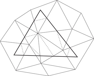
Figure 26.3Clip and retriangulate.

Let $C_{k + 1}$ $C_{k + 1}$ denote the collection of new simplices. A simplex of $C_{k + 1}$ $C_{k + 1}$ in σ is cut (in its interior) by at most ɛ0|H_σ| hyperplanes of H_σ, and hence of H. By induction, this produces at most $n ε_{0}^{k + 1}$ $n ε_{0}^{k + 1}$ cuts; therefore, $C_{k + 1}$ $C_{k + 1}$ is an $ε_{0}^{k + 1}$ $ε_{0}^{k + 1}$ -cutting. The only problem is that $C_{k + 1}$ $C_{k + 1}$ might be a little too big. The reason is that excess in size builds up from generation to generation. We circumvent this difficulty by using a global parameter that is independent of the construction; namely, the total number of vertices.

Note that we may assume that $| H_{σ} | > n ε_{0}^{k + 1}$ $| H_{σ} | > n ε_{0}^{k + 1}$ , since σ would otherwise already satisfy the requirement of the next generation. We distinguish between full and sparse simplices. Given a set X of hyperplanes and a d-dimensional (closed) simplex σ, let v(X, σ) be the number of vertices of $A (X)$ $A (X)$ in the interior of σ.

•The simplex $σ \in C_{k}$ $σ \in C_{k}$ is full if v(H, σ) ≥ c0|H_σ|d, where $c_{0} = ε_{0}^{2}$ $c_{0} = ε_{0}^{2}$ . If so, we compute an ɛ0-net for H_σ, and triangulate the portion of the net’s arrangement within σ to form an ɛ0-cutting of size $O (ε_{0}^{- 1} \log ε_{0}^{- 1})^{d}$ $O (ε_{0}^{- 1} \log ε_{0}^{- 1})^{d}$ . Its simplices form the elements of $C_{k + 1}$ $C_{k + 1}$ that lie within σ.

•A simplex σ that is not full is sparse. If so, we find a subset $H_{σ}^{o}$ $H_{σ}^{o}$ of H_σ that satisfies two conditions:

i.The canonically triangulated portion of $A (H_{σ}^{o})$ $A (H_{σ}^{o})$ that lies inside σ consists of a set $C_{σ}^{o}$ $C_{σ}^{o}$ of at most $\frac{1}{2} ε_{0}^{- d}$ $\frac{1}{2} ε_{0}^{- d}$ full-dimensional (closed) simplices.

ii.Each simplex of $C_{σ}^{o}$ $C_{σ}^{o}$ is intersected in its interior by at most ɛ0|H_σ| hyperplanes of H.

The elements of $C_{k + 1}$ $C_{k + 1}$ within σ are precisely the simplices of $C_{σ}^{o}$ $C_{σ}^{o}$ .

Lemma 26.3

$C_{k + 1}$ $C_{k + 1}$ is an $ε_{0}^{k + 1}$ $ε_{0}^{k + 1}$ -cutting of size $O (ε_{0}^{- d (k + 1)})$ $O (ε_{0}^{- d (k + 1)})$ .

Next, we explain how to enforce conditions (i) and (ii) for sparse simplices. To be able to distinguish between full and sparse simplices, we use a c0/2-approximation A_σ for H_σ of constant size, which we can build in O(|H_σ|) time (Theorem 26.3). It follows from Theorem 26.4 that

$\| \frac{v (H, σ)}{\| H_{σ} \|^{d}} - \frac{v (A_{σ}, σ) \|}{\| A_{σ} \|^{d}} \| \leq \frac{c_{0}}{2};$ $\| \frac{v (H, σ)}{\| H_{σ} \|^{d}} - \frac{v (A_{σ}, σ) \|}{\| A_{σ} \|^{d}} \| \leq \frac{c_{0}}{2};$	(26.1)

therefore, we can estimate v(H, σ) in constant time with an error of at most $\frac{c_{0}}{2} | H_{σ} |^{d}$ $\frac{c_{0}}{2} | H_{σ} |^{d}$ , which for our purposes here is inconsequential.

How do we go about refining σ and how costly is it? If σ is a full simplex, then by Theorem 26.3, we can compute the required ɛ0-net in O(|H_σ|) time. Within the same amount of time, we can also find the new set of simplices in σ, together with all of their incidence lists.

The refinement of a sparse simplex σ is a little more involved. We begin with a randomized construction, from which we then remove all the randomness. We compute $H_{σ}^{o}$ $H_{σ}^{o}$ by choosing a random sample from A_σ of size $c_{1} ε_{0}^{- 1} \log ε_{0}^{- 1}$ $c_{1} ε_{0}^{- 1} \log ε_{0}^{- 1}$ , for some constant c1 large enough (independent of ɛ0). It can be shown that, with probability at least 2/3, the sample forms an (ɛ0/2)-net for A_σ. By Lemma 26.2, $H_{σ}^{o}$ $H_{σ}^{o}$ is a (c0/2 + ɛ0/2)-net for H_σ; therefore, we ensure that (ii) holds with probability at least 2/3. A slightly more complex analysis shows that (i) also holds with probability at least 2/3; therefore (i,ii) are both true with probability at least 1/3. We derandomize the construction in a trivial manner by trying out all possible samples, which takes constant time; therefore, the running time for refining σ is O(|H_σ|).

Putting everything together, we see that refining any simplex takes time proportional to the total size of the incidence lists produced. By Lemma 26.3, the time needed for building generation k + 1 is $O (n ε_{0}^{- (d - 1) (k + 1)})$ $O (n ε_{0}^{- (d - 1) (k + 1)})$ . The construction goes on until we reach the first generation such that $ε_{0}^{k} \leq ε$ $ε_{0}^{k} \leq ε$ . This establishes Theorem 26.1.

From the proof above it is not difficult to derive a rough estimate on the constant factor in the O(ɛ^−d) bound on the size of an ɛ-cutting. A thorough investigation into the smallest possible constant was undertaken by Har-Peled [21] for the two-dimensional case.

26.3Applications

Cuttings have numerous uses in computational geometry. We mention just a handful: point location, Hopcroft’s problem, convex hulls, Voronoi diagrams, and range searching. In many cases, cuttings allow us to derandomize existing probabilistic solutions, that is, to remove any need for random bits and thus produce deterministic algorithms. Many other applications are described in the survey [5].

26.3.1Point Location

How do we preprocess n hyperplanes in Rd, so that, given a query point q, we can quickly find the face of the arrangement formed by the hyperplanes that contains the point? For an answer, simply set ɛ = 1/n in Theorem 26.1, and use the nesting structure of $C_{1}$ $C_{1}$ , $C_{2}$ $C_{2}$ , etc, to locate q in $C_{k}$ $C_{k}$ . Note that this can be done in constant time once we know the location in $C_{k - 1}$ $C_{k - 1}$ .

Theorem 26.5

Point location among n hyperplanes can be done in O(log n) query time, using O(nd) preprocessing.

Observe that if we only wish to determine whether the point q lies on one of the hyperplanes, it is possible to cut down the storage requirement a little. To do that, we use an ɛ-cutting for ɛ = (log n)/n. The cells associated with the bottom of the hierarchy are each cut by O(log n) hyperplanes, which we can therefore check one by one. This reduces the storage to O(nd/(log n)^d−1).

26.3.2Hopcroft’s Problem

Given n points and n lines in R2, is there any incidence between points and lines? This is Hopcroft’s problem. It is self-dual; therefore dualizing it won’t help. A classical arrangement of n lines due to Erdös has the property that its n highest-degree vertices are each incident to Ω(n^1/3) edges. By picking these n lines as input to Hopcroft’s problem and positioning the n points in the near vicinity of these high-degree vertices, we get a sense (not a proof) that to solve the problem should require checking each point against the Ω(n^1/3) lines incident to their nearby vertex. This leads to an Ω(n^4/3) running time, which under some realistic (though restrictive) conditions, can be made into a rigorous lower bound [22]. At the very least this line of reasoning suggests that to beat Ω(n^4/3) is unlikely to be easy. This bound has almost been achieved by an algorithm of Matoušek [23] with, at its heart, a highly intricate and subtle use of cuttings.

Theorem 26.6

To decide whether n points and n lines in the plane are free of any incidence can be done in n^4/3 2^O(log*n) time.

26.3.3Convex Hulls and Voronoi Diagrams

Cuttings play a key role in computing convex hulls in higher dimension. Given n points in Rd, their convex hull is a bounded convex polytope with O(n^⌊d/2⌋) vertices. Of course, it may have much fewer of them: for example, d + 1, if n − d − 1 points lie strictly inside the convex hull of the d + 1 others. It is notoriously difficult to design output-sensitive algorithms, the term designating algorithms whose running time is a function of both input and output sizes. In the “worst case” approach our goal is a simpler one: to design an optimal convex hull algorithm that runs in O(n logn + n^⌊d/2⌋) time. (The extra term n log n is unavoidable because sorting is easily embedded as a convex hull problem.)

Computing the convex hull of n points is equivalent by duality to computing the intersection of n halfspaces. A naive approach to this problem is to insert each halfspace one after the other while maintaining the intersection of previously inserted halfspaces incrementally. This can be done without difficulty if we maintain a canonical triangulation of the current intersection polyhedron and update a bipartite graph indicating which hyperplane intersects which cell of the triangulation. A surprising fact, first proven by Clarkson and Shor [24], is that if the halfspaces are inserted in random order, then the expected running time of the algorithm can be made optimal. By using an elaborate mix of ɛ-nets, ɛ-approximations, and ɛ-cuttings, Chazelle [25] showed how to compute the intersection deterministically in optimal time; his algorithm was subsequently simplified by Brönnimann, Chazelle, and Matoušek [16]; a complete description is also given in the book [10]. This implies the two theorems below.

Theorem 26.7

The polyhedron formed by the intersection of n halfspaces in Rd can be computed in O(n log n + n^⌊d/2⌋) time.

Not only does this result give us an optimal deterministic solution for convex hulls, but it also solves the Voronoi diagram problem. Indeed, recall [26,27] that a Voronoi diagram of n points in Rd can be “read off” from the facial structure of the convex hull of a lift of the n points into R^{d + 1}.

Theorem 26.8

The convex hull of a set of n points in Rd can be computed deterministically in O(n log n + n^⌊d/2⌋) time. By duality, the Voronoi diagram (or Delaunay triangulation) of a set of n points in Ed can be computed deterministically in O(n log n + n^⌈d/2⌉) time.

26.3.4Range Searching

Simplex range searching refers to the problem of preprocessing a set P of n points in Rd so that, given a query (closed) simplex σ, the size of P ∩ σ can be quickly evaluated. Variants of the problem include reporting the points of P ∩ σ explicitly or, assuming that each point p has a weight w(p) ∈ R, computing $\sum {w (p) | p \in P \cap σ}$ $\sum {w (p) | p \in P \cap σ}$ . The most powerful data structure for solving simplex range searching, the simplicial partition, vividly illustrates the power of ɛ-cuttings. A collection {(P_i, R_i)} is called a simplicial partition if

•The collection {P_i} forms a partition of P; and

•Each R_i is a relatively open simplex that contains P_i.

The simplices R_i can be of any dimension and, in fact, need not even be disjoint; furthermore the P_i’s need not be equal to P ∩ R_i. A hyperplane is said to cut R_i if it intersects, but does not contain, R_i. The cutting number of the simplicial partition refers to the maximum number of R_i’s that can be cut by a single hyperplane. Matoušek [28] designed an optimal construction, which happens to be crucially based on ɛ-cuttings.

Lemma 26.4

Given a set P of n points in Rd (d > 1), for any integer 1 < r ≤ n/2, there exists a simplicial partition of cutting number O(r^{1 − 1/d}) such that n/r ≤ |P_i| < 2n/r for each (P_i, R_i) in the partition.

To understand the usefulness of simplicial partitions for range searching, one needs to learn about partition trees. A partition tree for P is a tree $T$ $T$ whose root is associated with the point set P. The set P is partitioned into subsets P1,…, P_m, with each P_i associated with a distinct child v_i of the root. To each v_i corresponds a convex open set R_i, called the region of v_i, that contains P_i. The regions R_i are not necessarily disjoint. If |P_i| > 1, the subtree rooted at v_i is defined recursively with respect to P_i.

Armed with a partition tree, it is a simple matter to handle range search queries. In preprocessing, at each node we store the sum of the weights of the points associated with the corresponding region. To answer a query σ, we visit all the children v_i of the root and check whether σ intersects the region R_i of v_i: (i) if the answer is yes, but σ does not completely enclose the region R_i of v_i, then we visit v_i and recurse; (ii) if the answer is yes, but σ completely encloses R_i, we add to our current weight count the sum of the weights within P_i, which happens to be stored at v_i; (iii) if the answer is no, then we do not recurse at v_i.

It is straightforward to see that Lemma 26.4 can be used to construct partition trees. It remains for us to choose the branching factor. If we choose a large enough constant r, we end up with a partition tree that lets us answer simplex range search queries in O(n^{1 − 1/d + ɛ}) time for any fixed ɛ > 0, using only O(n) storage. A more complex argument by Matoušek [28] removes the ɛ term from the exponent.

With superlinear storage, various space-time tradeoffs can be achieved. For example, as shown by Chazelle, Sharir, and Welzl [29], simplex range searching with respect to n points in Rd can be done in O(n^{1 + ɛ}/m^1/d) query time, using a data structure of size m, for any n ≤ m ≤ nd. Matoušek [23] slightly improved the query time to O(n( logm/n)^{d + 1}/m^1/d), for m/n large enough. These bounds are essentially optimal under highly general computational models [10].

Acknowledgments

This work was supported in part by NSF grant CCR-998817, and ARO Grant DAAH04-96-1-0181.

References

1.Clarkson, K.L. New applications of random sampling in computational geometry, Disc. Comput. Geom. 2, 1987, 195–222.

2.Haussler, D., Welzl, E. ɛ-nets and simplex range queries, Disc. Comput. Geom. 2, 1987, 127–151.

3.Matoušek, J. Cutting hyperplane arrangements, Disc. Comput. Geom. 6, 1991, 385–406.

4.Agarwal, P.K. Partitioning arrangements of lines II: Applications, Disc. Comput. Geom. 5, 1990, 533–573.

5.Agarwal, P.K. Geometric partitioning and its applications, in Computational Geometry: Papers from the DIMACS Special Year, eds., Goodman, J.E., Pollack, R., Steiger, W., Amer. Math. Soc., 1991.

6.Matoušek, J. Construction of ɛ-nets, Disc. Comput. Geom. 5, 1990, 427–448.

7.Matoušek, J. Approximations and optimal geometric divide-and-conquer, J. Comput. Syst. Sci. 50, 1995, 203–208.

8.Chazelle, B. Cutting hyperplanes for divide-and-conquer, Disc. Comput. Geom. 9, 1993, 145–158.

9.Chazelle, B., Friedman, J. A deterministic view of random sampling and its use in geometry, Combinatorica 10, 1990, 229–249.

10.Chazelle, B. The Discrepancy Method: Randomness and Complexity, Cambridge University Press, hardcover 2000, paperback 2001.

11.Matoušek, J. Geometric Discrepancy: An Illustrated Guide, Algorithms and Combinatorics, 18, Springer, 1999.

12.Vapnik, V.N., Chervonenkis, A.Ya. On the uniform convergence of relative frequencies of events to their probabilities, Theory of Probability and its Applications 16, 1971, 264–280.

13.Sauer, N. On the density of families of sets, J. Combinatorial Theory A 13, 1972, 145–147.

14.Shelah, S. A combinatorial problem; stability and order for models and theories in infinitary languages, Pac. J. Math. 41, 1972, 247–261.

15.Chazelle, B., Matoušek, J. On linear-time deterministic algorithms for optimization problems in fixed dimension, J. Algorithms 21, 1996, 579–597.

16.Brönnimann, H., Chazelle, B., Matoušek, J. Product range spaces, sensitive sampling, and derandomization, SIAM J. Comput. 28, 1999, 1552–1575.

17.Komlós, J., Pach, J., Woeginger, G. Almost tight bounds for ɛ-nets, Disc. Comput. Geom. 7, 1992, 163–173.

18.Pach, J., Agarwal, P.K. Combinatorial Geometry, Wiley-Interscience Series in Discrete Mathematics and Optimization, John Wiley & Sons, Inc., 1995.

19.Matoušek, J. Tight upper bounds for the discrepancy of halfspaces, Disc. Comput. Geom. 13, 1995, 593–601.

20.Matoušek, J., Welzl, E., Wernisch, L. Discrepancy and ɛ-approximations for bounded VC-dimension, Combinatorica 13, 1993, 455–466.

21.Har-Peled, S. Constructing planar cuttings in theory and practice, SIAM J. Comput. 29, 2000, 2016–2039.

22.Erickson, J. New lower bounds for Hopcroft’s problem, Disc. Comput. Geom. 16, 1996, 389–418.

23.Matoušek, J. Range searching with efficient hierarchical cuttings, Disc. Comput. Geom. 10, 1993, 157–182.

24.Clarkson, K.L., Shor, P.W. Applications of random sampling in computational geometry, II, Disc. Comput. Geom. 4, 1989, 387–421.

25.Chazelle, B. An optimal convex hull algorithm in any fixed dimension, Disc. Comput. Geom. 10, 1993, 377–409.

26.Edelsbrunner, H. Algorithms in Combinatorial Geometry, Springer-Verlag, Berlin, 1987.

27.Ziegler, G.M. Lectures on Polytopes, Graduate Texts in Mathematics, 152, Springer, New York, 1995.

28.Matoušek, J. Efficient partition trees, Disc. Comput. Geom. 8, 1992, 315–334.

29.Chazelle, B., Sharir, M., Welzl, E. Quasi-optimal upper bounds for simplex range searching and new zone theorems, Algorithmica 8, 1992, 407–429.

^*This chapter has been reprinted from first edition of this Handbook, without any content updates.

..................Content has been hidden....................

You can't read the all page of ebook, please click here login for view all page.

Table of Contents for 26. Cuttings

Create new playlist

Sign In

Sign Up

Table of Contents for
26. Cuttings