
Step 1: Collect, Capture and Clean Data
Reminder of Major Initial Data Issues
These initial data steps
were mostly discussed in Chapter 4 and Chapter 9, and the basics of
collecting, capturing and cleaning data will not be covered in detail
here. The researcher is urged to remember that getting to know your
data well and ensuring it is cleaned and correct is crucial to all
statistics. The following are crucial summary points:
-
The crucial methodological design issues: The most important thing in research is to have the right sample and a correct and adequate set of variables which are put together in an appropriate model. This is also true of regression. No matter how well your model seems to fit and how strong your slopes, if the sample, variables or model are inadequate your analysis may be jeopardized or even meaningless.
-
Categorical data: If you have variables that are categorical data, they will need special treatment. In regression and most other similar techniques, we deal with categorical data in a special way. This topic is explained further in the next section.
-
Missing data: Missing data may be an issue for regression. I discuss the diagnostic steps and suggest a remedial solution in Diagnostic Issue #7: Missing Data below.
-
Multi-item scales: If you have multi-item scales, you can follow the steps in Chapter 9.
The end point of your
data steps is, of course, a datasheet with all your final variables
captured in rows and each observation in a row. Take a look at the
dataset “Textbook.Data05_Regression_Dummies” for the
final variables after combining multi-item scales.
Special Treatment of Categorical and Ordinal Predictors
Introducing Dummy Variables
Independent variables
can be categorical, that is,
the data value for each observation is not really a number but more
of an arbitrary indicator of membership in a certain category. For
example, gender (Male or Female) is binary categorical (there are
only two categories). Either words or any arbitrarily chosen number
can be used to indicate the person’s gender (e.g. 0 = male,
1 = female; 2 = male 1 = female, etc.) Categorical variables can also
have more than two categories, such as a variable measuring type of
company (categories might include services, retail, manufacturing,
etc.).
You can also use ordinal
variables indicating rank as independent variables.
In our case example the variable measuring size
of the customer has three increasing levels: small,
medium and big.
The problem with categorical
predictors in regression is that the values indicating category have
no numerical mathematical value. If 1=Auditing, 2=Tax, 3=Consulting
Services then you cannot say the 1 is “less than” the
3, as we would normally think of these values. Instead, the numbers
are really just tags. But, if you put the categorical variable into
a statistical program as numerical tags then the program will assume
that the data is in a true mathematical sequence. Even with ordinal
variables, where the numbers at least indicate relative position (higher
or lower rank than the others), because the distance between
the data points is mathematically meaningless, leaving the data as
it is, creates the problem that the statistical program will treat
it as a fully continuous variable.
Instead, when you have
categorical or ordinal independent variables like this, they need
to be rearranged in a special way (either by you or by the statistical
software). The most common method is to split up the one categorical
or ordinal variable into several dummy variables
[2]. Dummy
variables are columns of data containing only the values one (1) or
zero (0), where a value of ‘“1” indicates membership
in a specific category or level. For instance, in our example we have
customer size with three levels: 1 = Small, 2 = Medium, 3 = Big. You
would split this up into dummy columns where, for instance, “Small”
would have its own column. In that Small dummy variable, all the small
customers would be indicated with a “1”, all the medium
and big customers would be given a “0”. Similarly, you
might then also have a Medium column, where all the medium customers
would get values of “1” and all the rest would be “0.”
Note
that you require dummy variables for every category except for one
of the categories, which is omitted
. The reason for omitting one of
the categories is that the one left out is already inferred if a specific
observation has the value “0” for all other categories
(e.g. in the example above, if the big contracts are the omitted category,
then you know an observation is a big customer if it receives a “0”
for both the small and medium columns). The omitted category actually
becomes the reference category to which each of the other categories
is compared in the regression. Gender is another example: you do not
need one column for Males and another for Females. In a single column
you could code Females as “1”, and then you know that
the Males are “0.”
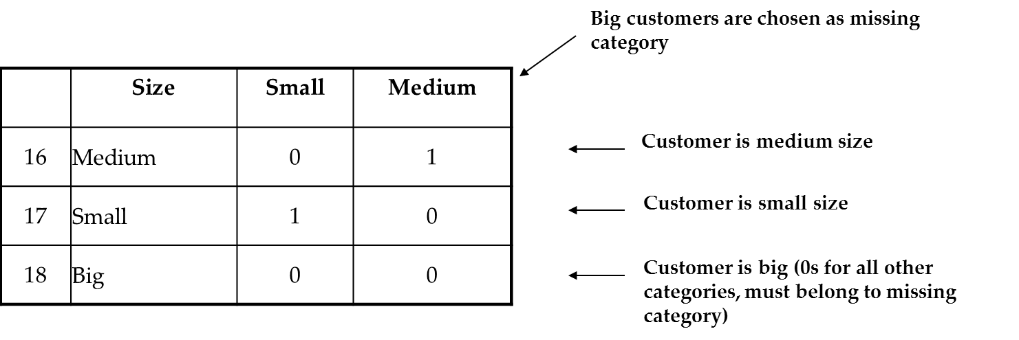
Figure 13.10 Illustration of coding categorical variables into dummy columns gives the case example using just three rows. Here we have
initially coded companies as small, medium and big. We choose one
group as the reference group (big, in this case), create dummy columns
for the other groups, and code these appropriately.
Figure 13.10 Illustration of coding categorical variables into dummy columns
Therefore, if you have
a categorical variable, the following needs to happen, either by you
doing it yourself in the dataset or through the statistical program
when you identify which variables are categorical:
-
Choose the reference category: Choose one of the categories as the reference category. This category will not be given a dummy variable. Choose a meaningful category, not the least important one.
-
Create dummy columns: Create one new column for each of the other categories which are not the reference category.
-
Naming dummy variables: I suggest giving each dummy variable a name that represents its category. For instance, if in a given dummy variable a “1” will indicate the premium license, call the variable “Premium” so that you can always identify what the variable represents. This may seem obvious but is not always so. Take gender, which is a binary dummy variable. You could assign a score of “1” to represent either male or female. If you call the column “Gender” then you will have to remember what the “1” refers to, but if you call the column “Female” (when “1” represents women) then you will never be confused. This is for your purposes: in actual reporting of the results, you can change the name back to gender if you like.
-
Dealing with small categories: Make sure all the categories have at least a decent number of representatives. You shouldn’t have any categories and therefore dummy variables without any representatives – this would just be all zeros and be meaningless. If you have categories with only a few members, consider whether it would be feasible to combine them (e.g. if you have columns for educational levels of people, but only have a few with masters and PhD degrees, consider combining them into one “postgraduate” column).
-
“Undefined other categories”: It is usually not very meaningful to have an “other” category as a dummy column. For instance, say you ask people to indicate educational levels such as high school, university undergraduate degree, and the like, and you include an undefined “other” category. I do not suggest having an “Other” dummy variable. Rather ask them to define exactly what they mean by “other” (e.g. if someone selects “other” and you require an explanation, the person might specify by writing “Chartered Finance Association qualification”). You could then decide that this equates to a diploma, and code the qualification under a “diplomas and equivalent” dummy variable. If you are stuck with undefined “other” answers, I recommend treating these as missing data.
-
-
Code the new dummy variables: Code the new dummy columns so that if the observation belongs to the category represented by the column, it receives a “1”; otherwise it receives a “0.”
You must create dummy
variables yourself in the data. There are two methods for achieving
this if you are using SAS:
-
You can create new variables in SAS. Chapter 6 explains how to do this. However, for the learning purposes of this book your data files come with the dummy variables already created (see “Data05_Regression_Dummies”), so you do not have to do this step yourself.
-
You can also create dummy variables in your original data before inputting it into SAS. For instance, in Microsoft Excel you could use functions to create dummy variables or copy the categorical variable and replace function to replace the one value with “1”s and all others with “0”s.
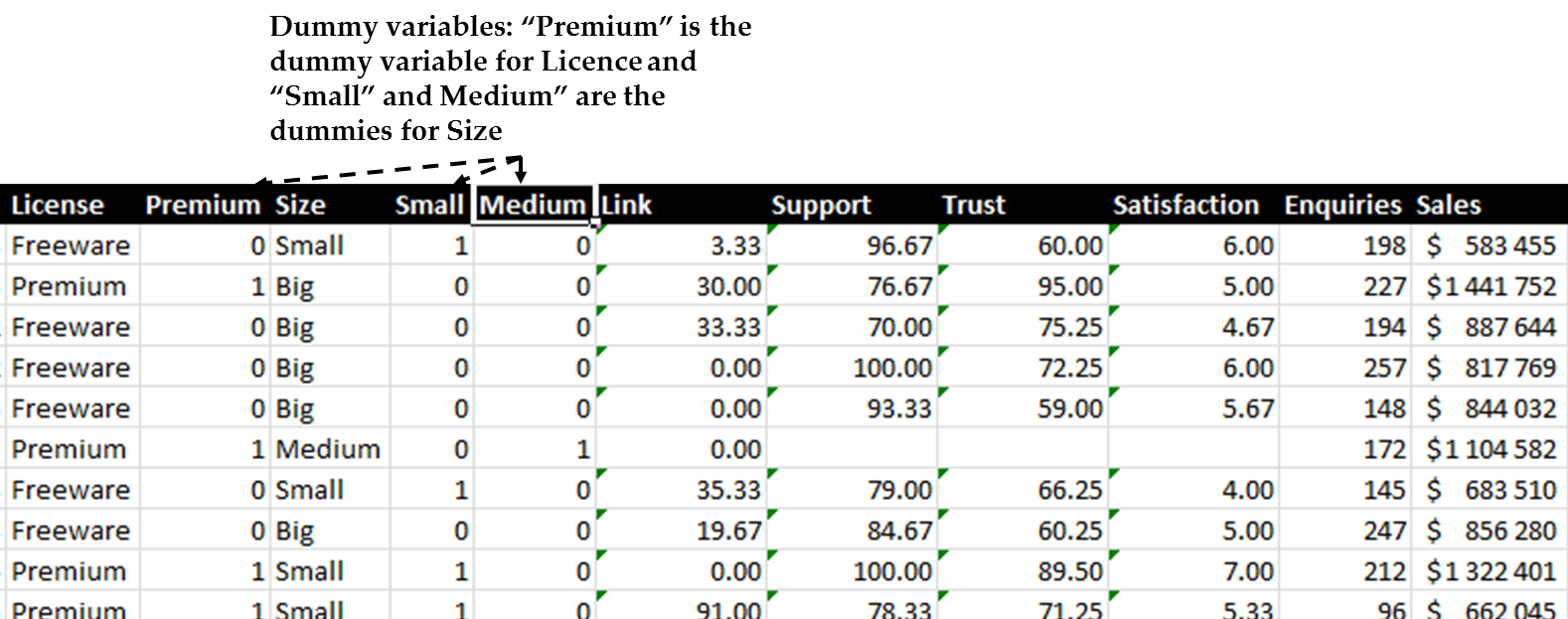
Figure 13.11 Example of data with dummy variables created shows an example of the regression case dataset with dummy
variables created.
Figure 13.11 Example of data with dummy variables created
One important question
you may have is how to treat single scale items on something like
a 1 to 5 point scale (e.g. a Likert scale from Strongly Disagree to
Strongly Agree). I discuss this below briefly.
Single Likert-Type Scale Items as Ordinal Predictors
When you have a single
scale item on something like a 1 to 5 point scale (e.g. a Likert scale
from Strongly Disagree to Strongly Agree) then, as stated previously,
many methodologists believe this to be ordinal data. When such data
stands alone as an independent variable, opinions are mixed as to
whether it’s safe to leave the data as it stands (a single
column with responses ranging from 1 to 5) or whether it would be
best to separate it into dummy variables (in the 1-5 scale case, either
using four dummy variables with one variable as a reference category,
or perhaps collapsing the data into a few dummy variables[3]). Of course, the best option is
never to have such data and either to use single-item response scales
with more continuous responses or to use aggregate scores from multi-item
scales. But, if you have to have such data, you will have to decide.
It may be a good idea to try both approaches and compare.
Having entered and prepared
our data, including dealing with the categorical variables, we can
now proceed to the regression analysis as discussed next.
Last updated: April 18, 2017
..................Content has been hidden....................
You can't read the all page of ebook, please click here login for view all page.