
Major Task #1: Data Manipulation in SAS
Introduction to Data Manipulation
Data manipulation
– in other words, changing data or creating new data –
is one of the most important tasks in practical business statistics.
After capturing data, it is rarely the case that the initial sheet
or database query is completely perfect for analysis. Often, changes
need to be made, for various reasons such as:
-
Imperfections in the original data that need to be fixed
-
The need to add new data
-
The need to combine multiple datasets
While you
can manipulate data in more basic spreadsheet programs like Microsoft
Excel, you can also do so in SAS, and far more simply, flexibly and
reliably. This book cannot cover much of the SAS data manipulation
universe, which is enormous and world-leading. The next few sections
can cover only a few salient topics. For a broader introduction to
these topics, the reader should consult texts such as Delwitch &
Slaughter (2012).
Creating New Datasets in SAS
As
a first topic, we often create new datasets in SAS programming code.
This section discusses the basics of doing this.
Of course, one way to
create new datasets in SAS is to import them from elsewhere, such
as importing Microsoft Excel files. Chapter 5 describes how to do
this. This chapter is more interested in dealing with data once it
is in SAS. To create or manipulate data in SAS we use a “DATA”
statement. Figure 6.4 Creating a new dataset in SAS shows
the outline of a data step for creating a new dataset SAS.
Figure 6.4 Creating a new dataset in SAS
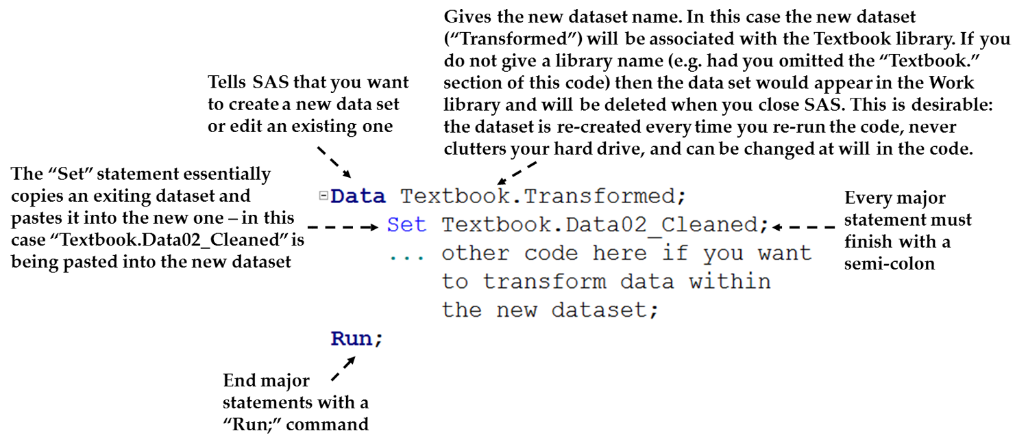
As seen in Figure 6.4 Creating a new dataset in SAS, if you wish
to create a new dataset you do the following:
-
Start with the keyword DATA, which tells SAS that you wish to create a new dataset.
-
Name the new dataset. Note the following:
-
Specify the name of a library and a dataset name, separated by a period (e.g. “Textbook.Transformed” in Figure 6.4 Creating a new dataset in SAS). The new SAS dataset will appear in the physical folder you have associated with this library. Of course, you have to have associated this library name with the folder beforehand, as described in Chapter 5.
-
There are basic rules for naming SAS datasets. This can be any name – in the code above we used the name “Transformed” – so long as it follows these rules:
-
A SAS name can contain from one to 32 characters.
-
The first character must be a letter or an underscore (_).
-
Subsequent characters must be letters, numbers, or underscores.
-
Blanks cannot appear in SAS names. If you want to separate parts of the dataset name, use underscores, e.g. “Dataset_03.”
-
-
If you leave out the library name and give only a dataset name (e.g. the “Data Transformed;” line in Figure 6.5 Example of creating new variables in the SAS DATA step below) then the new dataset will be created in the special “Work” library. In other words, calling the dataset “MyData” is the same as calling it “Work.MyData”. The “Work” library is automatically created as part of the SAS installation, and I explain it in more detail in the next section. Using this option is often desirable.
-
If you choose the same name and library as an existing dataset, then you will overwrite (i.e. replace) the original version of the dataset.
-
-
Populate the new dataset with initial data. There are two main choices here:
-
Populate the new dataset with data from another dataset. We frequently base the new dataset on the data from an existing dataset. Think of this as a copy and paste, i.e. you are copying data from an existing dataset into your new dataset. As seen in Figure 6.4 Creating a new dataset in SAS, we can do this by putting the line “SET <name of existing dataset>;” into a DATA step. In Figure 6.4 Creating a new dataset in SAS, we are using the SET statement to copy all the contents of the “Data02_Cleaned” dataset into the new “Transformed” dataset. In this code, both datasets are located in the “Textbook” library.
-
Enter raw data directly into SAS. You can also enter data literally in SAS in a DATA step. This book will not cover this direct data input option. I personally advocate importing initial raw data from a spreadsheet program such as Microsoft Excel.
-
-
If desired, manipulate the data. In the DATA step, we can manipulate the data in a great number of ways. Create New Variables or Manipulate Current Variables in SAS below describes more on such steps.
-
Other programming notes: As seen in Figure 6.4 Creating a new dataset in SAS, do not forget to place semicolons between major statements and add a “Run;” statement at the end before running.
Creating Temporary Datasets in the Work Library
The previous
section noted that if you do not give a library name as part of a
dataset name then you are automatically linking the dataset with the
special “Work” folder (so specifying “Profits”
is the same as saying “Work.Profits”).
The Work library has
a special property: all datasets contained within it are deleted when
you close SAS. This is desirable in many cases for two major reasons:
-
Datasets created in the Work folder do not clutter your hard drive or server, as they are deleted once you close SAS. However, because you can save the code used to create them, these datasets can be re-created every time you re-run the code. Programming code takes up far less space on a computer than data.
-
If you keep your original data and copy it to a Work library dataset, then changes you make to the new dataset do not affect the original data, which means you are never at risk of harming your original dataset.
This method of creating
datasets out of programming code only for the duration of your session
– and analyzing the temporary data as you need - is highly
efficient and often used by SAS analysts.
On the other hand, giving
a SAS library name other than Work causes the dataset to be stored
permanently in the folder associated with that library. This is, of
course, desirable in cases where you do wish to maintain a permanent
copy.
Create New Variables or Manipulate Current Variables in SAS
There
are many situations in business statistics where you wish to create
a new variable that is, in effect, a transformation of an existing
variable’s data. Here are some initial examples:
-
Creating an index such as a financial ratio (such as creating a price/earnings ratio from two columns containing price and earnings data, respectively).
-
Creating mathematical transformations of variables, such as a new variable that is the square root or log of another variable.
-
Using the birthdates of people to create a new column that, on a consistently updating basis, calculates their ages.
In addition, you can
change and manipulate existing variables in SAS.
In our main textbook
example, so far we have two major types of such tasks:
-
Creating new variables that reverse the data of reverse-worded survey questions. Specifically, Satisfaction04 is a reverse-worded survey item (see Chapter 4 and Chapter 9 for more on this), which required us to create a new variable that reverses its data.
-
Creating two new factor variables, which are the aggregation of multi-item scales. Trust and satisfaction ultimately needed to be created as factors which are an average of the individual multi-item scores. (Of course, we can’t do this step without having assessed internal reliability. Again, see Chapters 4 and 9).
One of the many things
SAS is brilliant at is data manipulation. You can manipulate data
by using the SAS point-and-click interfaces like SAS Enterprise Guide,
but it is quicker and easier to use code in programs like SAS 9 or
SAS Studio. The DATA step in SAS not only creates new datasets or
edits existing ones, but manipulates data columns or rows.
Figure 6.5 Example of creating new variables in the SAS DATA step shows a sample
SAS data step in which the new dataset is created based on an existing
dataset (specifically, we create a dataset called “Transformed”
in the Work library because no library is specified, and we copy and
paste everything from the Textbook.Data02_Cleaned dataset using the
SET statement).
Figure 6.5 Example of creating new variables in the SAS DATA step
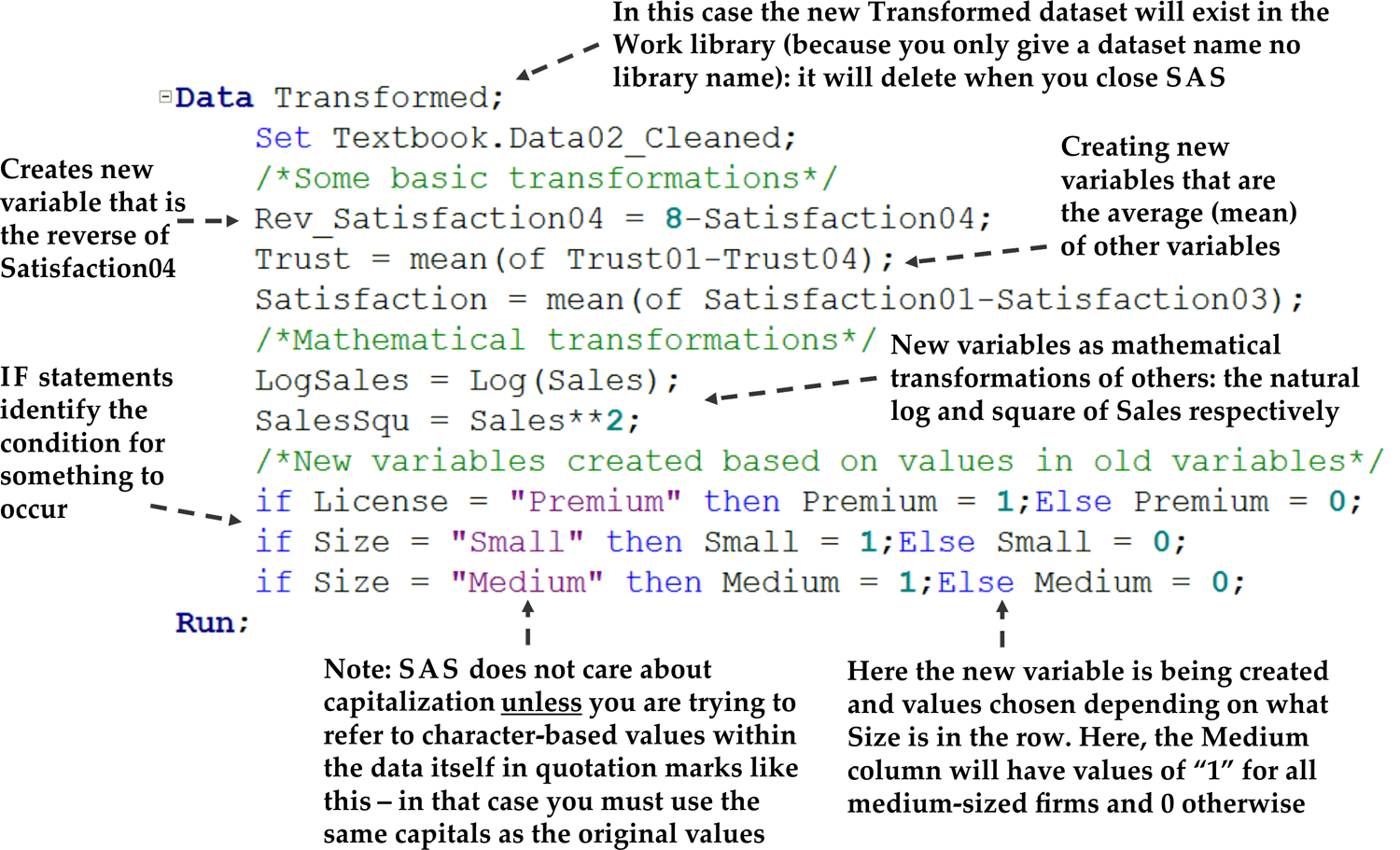
Then, each subsequent
line creates a new variable:
-
We create a new variable called “Rev_Satisfaction04” that takes the data from the existing variable Satisfaction04 and reverses it using the principles discussed in Chapter 4.
-
We create new variables called “Trust” and “Satisfaction” that are averages of some of the individual currently existing multi-item scale columns. Note the way the average works. Also, note here that I have only averaged the values for Satisfaction01-Satisfaction03; see Chapter 9 a little later for why.
-
We create two new mathematical transformations of the Sales variable, one the natural log and one for the square (each Sales number to the power of two).
-
We create several conditional variables using the IF-THEN concept, where the new variable only takes on a certain value if a given condition is true. In the first of these, we create a new variable called “Premium” that will have the value 1 whenever the currently existing License variable contains the value “Premium” in a row, and takes the value 0 for all rows where License is not “Premium.”
Take note of the following
programming notes about this sort of programming:
-
Take another look at the IF-THEN statements in Figure 6.5 Example of creating new variables in the SAS DATA step. Note here that this is the only situation in which capitalization counts in SAS. Take the example of the if License = “Premium” section of the code. Here, we are asking SAS to go look in the dataset for all rows where this exact condition is true including the exact capitalization of “Premium,” and then apply the result only in those rows. If there are also entries in the License column spelled “premium” then the above condition will not identify these rows. So, be careful of capitalization in these situations only.
-
As always, note that all statements are separated by semicolons and the entire set ends with a “Run;” statement.
You could do so much
more. For instance, you could create a new variable that is the sum
of other variables (replace MEAN in the above code with SUM). You
can identify rows to delete based on certain rules. SAS has an almost
endless set of possible variable manipulations – see the SAS
helpfiles (notably SAS/STAT 13.2 User’s Guide) for more.
Once you have told SAS
what you want to do, submit the code using the Run button as seen
above. Once you have done so, always check the log for errors and
always open the new dataset to check that it is right. (And then close
it: an open dataset in SAS cannot be replaced).
You can see the code
from this section in the textbook resources files, under “Code06
Manipulating data example.”
Combining Datasets
Often in the
business world, we need to combine two or more datasets together.
You can combine datasets side-by-side, one on top of the other, merge
them based on a match in a certain variable, and so on.
Let us look at one of
the most common examples: match merging. Imagine you are an organization
with the following two datasets:
-
A database of customer account data, where each customer is identified by a unique customer number.
-
A different database of customer satisfaction survey data. Again, each customer’s survey responses are identified by the customer number. Typically, only a limited subset of customers would have filled in the survey.
Now, let us say that
you wish to combine these two datasets so that you can link the data.
Each row needs to be matched up by customer number. You can do this
in SAS using the MERGE statement. See the following example:
Example Code 6.1 Example of merge matching data in SAS
Data Customers.Merged;
	Merge Customers.Accounts Customers.Survey2016;
	By Customer_ID;
Run;
There are many nuances
and complexities to combining datasets – for instance, to match
merge by a common variable as I show above, both datasets must be
sorted by the common matching variable (i.e. you would have to sort
both of the above datasets by Customer_ID). For more on combining
datasets, reference the SAS helpfiles or books such as Delwitch &
Slaughter (2012).
This basic understanding
of SAS data manipulation will help us in various parts of the rest
of the book, since data manipulation is frequently required in statistical
analysis.
Last updated: April 18, 2017
..................Content has been hidden....................
You can't read the all page of ebook, please click here login for view all page.