
Look for Patterns in the Data (Fit)
Introduction
The primary job of the statistician is to look for patterns in the data that he or
she has gathered. We call this the ”fit” step. There are various options as discussed
in the next few sections, depending on the number of variables and type of statistic
you are seeking.
Single Variable Patterns
You might be interested in the way the data is arranged in a single variable.
For instance, say that you have a single variable composed of the tenures (length
of employment in months) of employees in your company. Your initial interest might
be in understanding the way tenures are distributed. You may find that the vast majority
of the employees are arranged in a distribution around a tenure of about 26 months
(the median), and 90% have been with you for about 7 years or less. However, there
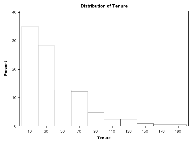
are some employees who have been around for as long as 16 years. Figure 11.2 Examining the distribution of a single variable shows a histogram graph of the tenures in different bands (measured in months) –
as you can see, there is a long (although small) tail to the right where the longest-serving
tenures are.
Figure 11.2 Examining the distribution of a single variable
Why would you want such an analysis? Perhaps the company is undertaking a long-term
retention program and wishes to keep track of this distribution over time to see if
they can shift the median and average tenures to the right (greater retention) and
perhaps achieve other aims.
Multivariate Patterns
You might also be interested in the way data is arranged between multiple variables
(we call this multivariate statistics).
For instance, in Chapter 3 and Chapter 8 we learned about a simple illustration, the
correlation between two variables.
If a correlation is to exist, then the data needs to have the type of pattern discussed
in the correlation section of Chapter 8, namely, that on average, when an observation
has a high score on one of the variables, it either has a high score on the other
variable (a positive correlation with upward linear pattern, like that seen in the
first panel of Figure 11.3 Reminder of data patterns underlying correlations) or a low score on the other variable (a negative correlation with downward linear
pattern, like that seen in the second panel of Figure 11.3 Reminder of data patterns underlying correlations).
Figure 11.3 Reminder of data patterns underlying correlations

Investigating a Theory Versus Data Mining
Two Paradigms
There are two very different paradigms for examining patterns in or between constructs,
namely, modeling a preconceived idea that you have about the data versus data mining.
Modeling Preconceived Ideas about Data
Modeling preconceived ideas about data is where you look for patterns that you have predetermined might or should exist,
so it is idea-based analysis. Here the researcher thinks in advance of analysis about
what patterns he or she expects to find in the data. Optimally the researcher builds
a strong theory regarding the analysis at hand, including whatever he or she expects
to find in the focal variables. If you have predictor variables, you typically have
predetermined ideas about how they explain or predict the focal variables, and whether
they interact with each other. Such theories are often based on the thinking expressed
in books and articles written by experts and thinkers in your field, who deeply consider
the knowledge in an area and suggest theories. If you want to do something in the
area, you may read these theories and then test to see if they’re right. You may merely
use your own rational logic to think in advance about what you may find.
For example, say that you are doing research on employee turnover in your company,
a focal variable you would love to explain and predict better. You are especially
interested in whether turnover differs by employee performance, since losing top performers
is a real concern. You read up on turnover literature and find out that theorists
such as Jackofsky (1984) and others suggest that low and high performers are more
likely to leave and mid-level performers are the least likely to leave. You may then
set out to look for this pattern in your data.
Data Mining
Data mining is essentially looking for any patterns that data can show you. Data mining is quite different, because here the researcher does not have a predetermined
theory about what patterns might be found in the data. Rather, data mining usually
involves using computer algorithms to search out patterns, which are then analyzed
by the researchers after they have been found. Data mining is more often used when
there is a lot of data – notably that gathered by companies – and where there is no
background theory.
For instance, financial services companies keep lots of data about their customers
and are interested in focal variables such as defaults on loan repayments and value
of transactions. They routinely data mine this for patterns, not necessarily knowing
in advance what they will find. Say that you find out that people who pay tithes to
churches are far less likely to default on loans. If a consistent pattern, this may
be used as part of the decision process behind whether to offer loans.
Comparing Theory-Based Analysis & Data Mining
It is absolutely critical that researchers think deeply about the advantages and disadvantages
of each of these approaches. Data mining seems seductive at first because you might
find patterns you didn’t expect that are gems and lead you to new ideas or strategies
in the future. However, consider the following:
-
Choosing the right variables: When you have a theory you then have a guide as to what constructs and data you need, including focal, predictor and environment variables. You set out to gather the appropriate data for these using the best methods possible. In data mining, all too often you are given data that already exists. You then run the risk that you don’t choose the right variables to analyze, or that you don’t have the right environmental controls or predictors, and the patterns you find are suspect as a result.
-
Random patterns: Data is always random to some degree, and any pattern you find you may not find again. At least when you have a theory, you have reasons for the patterns and therefore some faith in why they are there (if they are). Data mining, however, runs the risk of finding patterns that are random flukes that are not to be repeated. You can do further studies to corroborate patterns you find in data mining, but that might be difficult. You should build a theory at this stage about what you found and why.
-
Reasons for patterns: As stated above, when you have theory you hopefully know why your patterns exist. Data mining runs the risk of finding a pattern but not knowing why you found it.
-
Implications of patterns: When you look for specific predetermined patterns, you almost certainly do so for a good reason: you knew why you wanted to do the study and what good it would do you. With data mining, you run the risk of finding patterns but not knowing what they mean or what to do about them.
Having said this, data mining is a great tool that is increasingly used by companies
and others, especially when you have large amounts of data and are not sure of where
the important or worthwhile patterns or starting points are.
Plots Versus Statistical “Fit” Measures of Patterns
So far we have discussed the concept of finding patterns in terms of graphical analysis.
Analysis of graphs is often not good enough for multivariate analysis of patterns;
sometimes it’s not even possible. When you have multiple variables interacting together,
graphics are often too difficult to understand. (You can often look only at three
variables together in a graph; what if you have twenty?)
Also, graphs are debatable. Although the first panel in Figure 11.3 Reminder of data patterns underlying correlations seems to show that the data cloud between variable 1 and variable 2 goes in an upward
direction (suggesting a positive correlation), it is also spread out. Is it a strong
correlation or not?
Sometimes you get formalized, numerical, statistical tests of whether there is a pattern
to be found in the data. We often call these ”fit” statistics. Therefore, to look
at patterns in data you usually want a combination of numerical statistical tests
and graphical analysis.
How Patterns Are Really Found: Fitting Mathematical Models
Fitting Actual Data to Exact Mathematical Shapes
As stated above, looking for patterns by visual examination of data is often too difficult.
More often, we compare the distribution and relationships in data versus various specific
definite relationships as defined by mathematical models.
The mathematical shape that we compare the actual data against is essentially a precise
expectation of a given pattern – a perfect pattern. Take for example Figure 11.4 Example: comparing data against mathematical shapes for fit, which is again tenure data for a company. Perhaps we wish to test whether or not
this data follows the precise mathematical shape seen in the black line in Figure 11.4 Example: comparing data against mathematical shapes for fit, which represents a normal distribution. (The left tail of the distribution has been
cut off by SAS here to make the graph area work).
Figure 11.4 Example: comparing data against mathematical shapes for fit
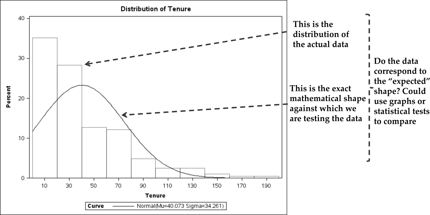
The question in Figure 11.4 Example: comparing data against mathematical shapes for fit is not whether the actual data will exactly fit a perfect shape: data is always at
least a bit random so it never fits any exact shape perfectly. However, the question
is whether the data fit sufficiently tightly to the exact mathematical ideal to be
deemed close enough, so that we can have reasonable certainty that we have found the
pattern.
In statistics this correspondence between an exact mathematical ideal shape and actual
data is called ”statistical fit” – usually, this is how we really confirm or disconfirm
the existence of patterns in data. Therefore, to test fit we usually do the following:
-
Generate the mathematical shape in the best possible way in the data.
-
Check using graphs or statistical measures whether the data lies close to the exact shape.
-
If the data lies close to the exact shape, assume you have found this sort of pattern in the data, and move on to interpreting the pattern that you have discovered.
-
If the data does not lie close to the exact shape, assume that this type of pattern is not found in the data. Do not assume that there is no pattern – there may be another type of pattern. I expand on this below.
The next section gives a somewhat tongue-in-cheek metaphor for the process of fitting
models to data.
Metaphor for Fitting Statistical Models: Constellations
I like the metaphor of star constellations as a picture for data fitting. Think of
the stars as data. Nothing in the stars is an exact pattern. But, sometime in history,
some (possibly stoned?) Greek turned around to his friend and went “Dude! Those stars
over there look like a lion!” Figure 11.5 The stars (data) of the constellation Leo shows stars in the constellation Leo – you might think of these as actual data.
Figure 11.5 The stars (data) of the constellation Leo

Figure 11.6 Overlaying a hypothetical picture of a Lion over the stars of Leo shows a hypothetical picture of a lion laid over the stars – you may think of the
picture as an exact perfect model of a lion. The stars do not follow the lion picture
exactly, but perhaps they come close enough to give agreement that a lion is a good
approximation of the pattern.
Figure 11.6 Overlaying a hypothetical picture of a Lion over the stars of Leo

Your task would be to determine how closely the data (or stars) really fit to the
picture of the lion. Plots and certain fit statistics would typically be available
for this. If the data does not fit a lion, perhaps there is no shape, or perhaps some
other shape will fit well (a dog? a car?) The final shape that fits may or may not
be helpful to you – that would be another question, and is discussed in the next major
step on interpretation.
In a more typical mode, the next sections give three statistical examples of formally
testing for fit of a pattern in data[1].
Example 1: Testing Data for a Straight Line Shape
Correlation and regression-type statistics mostly look for straight line (linear)
relationships in data. Chapter 13 deals with such relationships in far more depth,
but let us get a more general idea here. Say you have only two variables, sales and
age, and you think age might affect levels of sales. (Sales is therefore your focus
variable, and age is a predictor variable.) You might also have some other control
or environmental variables in the background. Figure 11.7 Fitting a straight line to data shows an example of age versus sales data (each dot represents a salesperson situated
above his or her age and next to his or her sales averages). The dotted line represents
an exact straight line.
Figure 11.7 Fitting a straight line to data
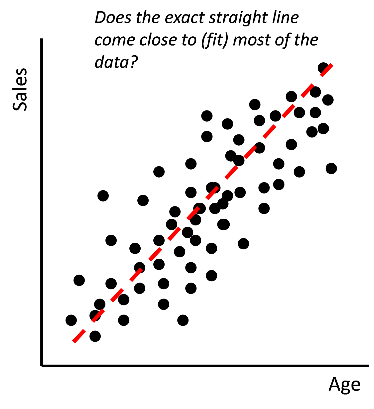
Focus on the dotted line that is the hypothetical, perfect linear relationship between
age and sales. If you think back to your school mathematics, you probably learned
that the exact, mathematical equation for a straight line is Y = mX + c or something similar. In this example, Y would be the dependent variable Sales, and
X would be the predictor variable Age. There are also two numbers m and c that are
condensed descriptions of the shape of the line (we call these ”parameters” or ”coefficients”):
c indicates the intercept of the line and m indicates how steep the line is (its slope).
So, the dotted line is represented by some version of the equation Sales = m(Age)
+ c where m and c are parameters that must take on exact values. For instance, in the example here, the dotted line
might be defined by the equation Sales = 7,200(Age) + 24,500. Here, we care most for
the slope (steepness) of the line. The size of the slope parameter (which is $7,200
here) is the key thing.
Your first question – the fit one – is “does most of the data lie close to this exact
straight line?” If so, you can go on to interpret what the straight line tells us.
What does the $7,200 slope tell us? Chapter 13 on regression goes on to discuss these
straight-line equation concepts in far more detail.
Example 2: Testing Data for a Normal Distribution
Recall from Appendix A of Chapter 7 that one basic example of testing a dataset for
a pattern is comparing the distribution of a variable against normality. If the variable
is normal it will follow a normal-like curve.
In that Appendix, I discuss that you can visually check the graph for differences
between the perfect mathematical model of the black normality line and the actual
data. However, you would probably want more confirmation, by using statistical measures.
The shape of a normal curve can be condensed into just two basic statistical measures,
namely ”skewness” and ”kurtosis.”
-
Skewness: A perfect normal distribution has skewness = 0. Visually, the tenure data in Figure 11.2 Examining the distribution of a single variable is at least a bit skewed to the right, i.e. positive skew. To formally test this we can look at the data’s skewness score. Data with skewness = 0 is equally distributed around the middle (the benchmark) like a normal distribution. The tenure data has skewness = 1.16 . The question to be asked is whether 1.16[2] is sufficiently far away from the zero benchmark to suggest that the data does not fit a normal distribution. For this, sometimes you get debatable cut-offs (e.g. “skewness outside the range of +-1 may indicate significant non-normal shape”[3]), and sometimes you get more sophisticated tests of a nature introduced in the next chapter. Ultimately all these tests help you answer the question ”does the data fit my pattern,” or in the example ”is this data normally distributed with close to zero skew, or skewed enough to reject normality?”
-
Kurtosis: A perfect normal distribution has a certain height and shape (in SAS the variable would have a kurtosis score of 0). Again, you test the actual data’s kurtosis score against the benchmark of zero either by applying cut-offs (in this case many authors suggest a cut-off of +-3) or through more sophisticated tests[4] . The tenure data has a kurtosis score = 3, so we may conclude that there is a likely departure from a normal distribution shape.
In summary we undertook the following process as discussed earlier:
-
You have one or more variables (in this case tenure) and want to test the actual data shape against a certain pattern (in this case a normal distribution);
-
As in Figure 11.4 Example: comparing data against mathematical shapes for fit you compare the data against the perfect mathematical distribution (in SAS, perfect normality is represented by the black line and skewness and kurtosis = 0).
-
The actual tenure data has its own (imperfect) skewness and kurtosis – the real question is whether these are significantly different from zero to indicate non-normality. For the tenure data you got skewness = 1.16 and kurtosis = 3.00. If we buy into cut-offs for skewness of +-1 and kurtosis of +-3 for significant deviations from normality (which are debatable), then we would reject a normal pattern here.
-
Both the graphical and statistical comparison of tenure data against the normal distribution seems to indicate that the data does not fit this type of pattern well. As discussed next, this does not mean there is no pattern, just that the one we tested is not a good fit here.
Example 3: Fitting a Complex Mathematical Equation to Data
Every year, when the Nobel prizes are awarded, a group of jokers in the scientific
community also award the “IgNobel” awards for research that should never have happened
or should never be repeated. In 2002 the IgNobel award in mathematics went to K.P.
Sreekumar and G. Nirmalanof for coming up with an equation for estimating the total
surface area of Indian elephants. You laugh? Well, true, if you tried to test almost
any actual dataset against this equation, it would not fit … unless your data was in fact measurements from the surface areas of Indian elephants! In that case, you would in fact probably have the right equation, and you would
be able to test whether the equation does a good job of fitting the data.
In summary, we often test for patterns in data by comparing the data to a hypothetical
perfect shape. Note, again, that although I’ve used pictures above as one way of assessing
fit to a shape, you cannot always do so, and formal statistical fit tests with given
rules are more often used for this purpose. You will learn about several such fit
statistics through the course of this book.
It is very important that you don’t misinterpret the fact that data fits to a pattern
for importance or usefulness of the pattern. Step 3: Interpret the Pattern discusses the very different step of interpreting the pattern.
Intermediate Fit Statistics vs. Final Statistical Parameters and Coefficients
So far, I have said that when looking for patterns in data you get a certain class
of statistical tests or numbers – often called fit statistics – that help you to do
this.
However, the point that has been made above is that assessing whether your data has
a certain pattern or not is only a step along the path. The characteristics of the
pattern – if there is one – are what finally count, not the fact that there is a pattern.
The characteristics of the pattern are also described by statistical numbers, and
it is these final statistical parameters and coefficients that we care about.
Readers often get confused between the intermediate fit statistics that help identify
patterns and the final statistical coefficients that actually describe the pattern.
In any advanced statistical techniques there are pages of numbers. Much of the output
is often the intermediate fit assessment just telling you if there is an appropriate
pattern in the data or not. But don’t forget that ”holy grail” of the final few statistics
that describe the pattern itself, if there is a pattern, and therefore tell you what
you wanted to know about the world.
In case this still seems a little confusing, let me give a metaphor for the difference
between intermediate fit statistics and final statistical parameters. Say that you
want to buy a car. You ultimately care about the combinations of price, age, type,
safety rating, etc. It is the statistics on these final characteristics (price etc.)
that you care about. Being an individual, you may have preferences on the optimal
combination of price, age, and the like.
Now, there are hundreds of thousands of cars for sale out there. Say that you download
some database of cars for sale. You could look through it one record at a time, but
this might be tough. Instead, you write a computer algorithm that identifies all the
cars that are close to your preferences (this is a bit like data mining).
The algorithm might tell you that a certain Subaru is 88% close to your specifications.
This is an intermediate fit statistic that helps you understand fit of data to your
preferred pattern. The 88% does not actually tell you what the price is exactly, or
if the high score has to do with safety more than age, for example. However, the 88%
fit statistic has helped you along the way. Now you can look at the actual price,
safety and other characteristics that are the final statistical coefficients of interest.
Don’t Force Patterns that Are Not There!
Researchers too often want to see or force patterns that are not there, usually because
they had a previous opinion about what was ”right” or desirable to see. (Actually
this is a bigger risk for theory-based research than data mining.) My favorite expression
for this is “torturing the data until it confesses!”
Here’s one possible example of torturing the data until it confesses. In a fascinating
New Yorker review, Lehrer (2010) discusses research findings about things like the effectiveness
of second-generation antipsychotic drugs, which are big business for pharmaceutical
companies. He points out that the findings of drug trials were initially seemingly
strong, leading to the drugs’ approval and high sales. However, the more researchers
studied the drugs, the more that the effects seemed to dwindle. This has happened
in other scientific areas as well. One explanation may be that the scientific community
wants to find results when it both does studies and when it chooses what to publish.
So, researchers may “cherry pick” only strong results from arrays of weak to strong
tests, or only results that corroborate their theories. Then, only (possibly fluke)
strong results get published early on. Other studies may have found weak effects but
these were not interesting enough to get published. Ultimately the published studies
seem to show support for the drug, whereas possibly, the effect is found only sometimes
at high dosages of the drug, and in fact maybe not very often.
It is especially common that researchers want to see linear relationships of the positive
or negative correlation type, as we will see later in the section on regression type.
Here are a few examples of this type of bias. ”Surely when satisfaction of employees
goes up, turnover will go down?“ ”Surely when we spend more on advertising, we will
see an increase in sales?”
Of course, the world is not necessarily as simple as we think or want it to be:
-
Sometimes patterns in data that we expect to see (distributions, relationships, etc.) simply do not exist, run in the opposite direction to that expected, or are too weak to take seriously.
-
Perhaps such patterns might exist but there is a good reason for not seeing them in this study. Possibly we’ve not got the right data to find the patterns in the first place. (Do we have the right variables to express our constructs? Do we have the right measurements of those variables?) Or, have we not yet tested for the right pattern in the data?
Next I discuss what to do if you do not find an expected pattern in the data.
What to Do When You Don’t Find Your Expected Pattern
When we don’t see the patterns we expected – or the patterns are expressed far more
weakly than we expected – we have choices, and we must face these bravely.
First, if we were doing theory-based research, we might need to discount the theory.
Don’t rush to this conclusion, but don’t be afraid of it. If we had a basic theory
in the first place but we find that the data doesn’t support it, we can discount this
theory, i.e. decide that it’s wrong. If we do so, we should come up with an alternative
set of explanations about why what we thought would happen has not in fact happened.
It is usually up to other researchers or further research done by yourself to corroborate
your lack of the expected finding and then to deliberately test and confirm alternative
explanations.
Here’s an example of not finding a pattern and looking for alternative theory. The
on-the-job training theory of Gary Becker (Nobel prize-winning economist) predicts
that when training is general (the skills can be shared across multiple or all firms)
that the employee will pay for such training (Becker, 1975) because employees can
either use the skills to move to a better job or negotiate current wages up. Much
research went into this: basically Becker was at least partially wrong since firms
are found on average to pay for substantial amounts of general training. Many researchers
such as Acemoglu and Pischke (1999) and Boom (2005) have offered alternate explanations
and theories. The research process went from theory (Becker’s theory on general training and who pays for it) to constructs (payment towards training, predicted by type of training, possibly controlling for
environmental variables) to data (actual measures of the constructs) to patterns in the data (whoops, not as expected because general training is not even nearly paid for completely
by employees) to a model (suggestions for an alternative model since the data is not supportive) to implications and further research.
If you are data mining without theory, perhaps you should discount the exercise. If you are data mining without a pre-set expectation of the findings and you cannot
find patterns of discernible value, you are probably less prone to trying to find
something in particular that is not there (because in data mining you didn’t expect
to find anything in particular). However, at some stage you should terminate the data
mining exercise or the current dataset! Although you could add complexity to the algorithms
being used in the data mining to try to find patterns (you may indeed find patterns
not discovered before), at some stage this approach becomes prohibitive.
Perhaps you should gather new data. One other option is that the data you used was badly measured or in some other way
inappropriate, and that the theory or data mining exercise still holds. The researcher
may revisit the way that the old data was put together or gather new data and continue
to test or mine it for the same study or algorithms.
Remember what we said at the beginning, finding a pattern is not always enough. Ultimately,
the patterns need to mean something. That’s why there is an extra step – that of interpreting
the pattern. This is discussed in the next section.
Last updated: April 18, 2017
..................Content has been hidden....................
You can't read the all page of ebook, please click here login for view all page.