
Chapter 16. Survey of Real-Time 3D Graphics Platforms
16.1. Introduction
Now that you’ve seen the core ideas that let us use computer graphics to make pictures, we’re going to describe to you the variety of approaches that have been developed to encapsulate this knowledge. Such approaches have the benefit of isolating the programmer from the details of the graphics hardware, which helps with maintainability of programs. They also let application developers concentrate on things specific to their application domain, rather than the way that images are presented to the user. The variety of approaches available is due, in part, to the pattern of hardware development, which is where we’ll begin our survey.
As impressive as the rate of improvement in commodity CPUs has been during the past four decades, the evolution of graphics hardware has been even more remarkable. Hardware-based graphics acceleration—removing the burden of executing the 3D pipeline from the primary processor by offloading it onto a peripheral—was first commercialized for vector displays in the late 1960s and for raster displays in the 1980s. Rendering pipelines moved from software to raster graphics hardware via the development of geometry- and pixel-processing chips that were integrated into graphics workstations built by high-end real-time 3D graphics vendors such as SGI and Evans & Sutherland, and mid-level-performance raster graphics was provided by workstation vendors including Apollo and Sun Microsystems. These devices were expensive, affordable only to academic and corporate institutions. The maturation of this technology into a true commodity, available on personal computers, took place in the mid-1990s in the form of graphics cards featuring cheap but powerful GPUs (described in Chapter 38).
Since each brand/model of GPU has its own native instruction set and interface, a standard API providing hardware independence is essential. The two dominant APIs providing this important abstraction layer are Microsoft’s proprietary Direct3D1 (on Windows platforms for desktop/laptop, smartphone, and gaming hardware such as Xbox 360) and the open source cross-platform OpenGL.
1. Direct3D is the 3D graphics portion of the umbrella suite of multimedia APIs that is known as DirectX. Note that some 3D-related publications will use the two names interchangeably, but the proper way to refer to the 3D functionality is to use the term “Direct3D” or the abbreviation “D3D.”
The goal of these low-level platforms is to provide access to the graphics hardware functions in a hardware-independent manner with minimal resource cost; they are thin layers above the graphics hardware device drivers. A key characteristic is that they do not retain the scene; instead, the application must respecify the scene to the platform in order to perform any update of the display. These immediate-mode (IM) platforms thus act as conduits to the graphics hardware, translating a device-independent stream of graphics instructions and data into the proprietary instruction set of the underlying GPU.
You as a developer have the choice of directly using a low-level IM API—which places the application close to the hardware, allowing maximum control—or using a retained-mode (RM) middleware platform (such as WPF) that offers the convenient abstraction of a scene graph. RM platforms—described in greater detail in Section 16.4.2—create opportunities for automated performance optimization, and simplify many development tasks by making it easier to express complex constructions. However, when you use an RM platform, you lose the potential for peak performance and may experience delays in access to the latest hardware features when waiting for the next release of the middleware. It is usually a good idea to work at the highest level practical for your application, and use a limited amount of lower-level code for performance-critical features.
It is important to note that the architecture of graphics hardware is in flux, as GPUs become more powerful and more general-purpose. The GPU is rapidly morphing into what might be called a Highly Parallel Processing Unit, which has already brought ray tracing onto commodity graphics hardware and into the realm of real-time rendering. Keep in mind that our focus here is on platforms built using current GPU polygon-rendering architectures.
16.1.1. Evolution from Fixed-Function to Programmable Rendering Pipeline
Graphics hardware and IM APIs have been co-evolving for several decades, each influencing the other. New features on the hardware side have, of course, required API enhancements for access. Simultaneously, developer identification of bottlenecks and limitations in the IM layer and the underlying hardware produces feedback that leads to innovations in graphics hardware. The co-evolution has, over time, caused a major paradigm shift in the IM layer’s functionality, as exhibited in Figure 16.1, whose focus is on the evolution of the two most pervasive IM platforms on commodity hardware.
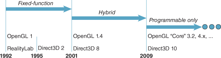
Figure 16.1: Evolution of two important commercial real-time 3D graphics platforms: OpenGL and Direct3D.
16.1.1.1. The Fixed-Function Era
Commodity graphics acceleration hardware in the early/mid-1990s implemented fixed-function (FF) pipelines (similar to WPF’s) using industry-standard non-global lighting and shading models (Phong or Blinn-Phong lighting, Gouraud or Phong shading), and depth-buffer visible surface determination as described in Section 36.3. The modules in the pipeline were configurable via parameters, but their algorithms were hardwired and could not be customized or replaced. Thus, the IM platforms in that era were focused on providing access to the FF features, and as new features were introduced in successive hardware releases, the IM APIs expanded to provide access.
16.1.1.2. Extensibility via Shaders: The “Hybrid Pipeline” Era
As the CG community demanded ever-higher levels of control over the rendering process and greater access to GPU capabilities, the popularity of shaders surged in the early 2000s—almost a full two decades after their introduction in a seminal 1984 paper by Rob Cook and pioneering implementation as part of Pixar’s RenderMan software developed by Hanrahan et al. The term “shader” is misleading, as it would seem to restrict its utility to just surface-color determination—in actuality, the technology encompasses many stages of the rendering pipeline and the term thus refers to any programmable module that can be dynamically installed into the 3D rendering pipeline.
For many years, shader programming had a steep learning curve due to its assembly-language specification; however, in the 2003–2004 time frame, shader programming became more accessible with the development of high-level languages (similar to C) like HLSL/Cg (from a Microsoft/NVIDIA collaboration) and GLSL (introduced in OpenGL 2.0, designed by the OpenGL Architecture Review Board).
The IM layer initially treated shader support as an add-on to the FF pipeline, and for many years, fixed and programmable features co-existed, with applications using the FF pipeline when appropriate and installing supplementary shaders as needed. For example, an animation house working on a movie could use the hybrid pipeline to facilitate real-time tests of scenes before moving on to expensive ray-traced renderings; the availability of shaders could be used to allow the real-time rendering to have at least some special effects such as a water-surface effect that cannot be achieved with the FF pipeline.
16.1.1.3. The Programmable Pipeline
As would be expected, reliance on the FF pipeline has decreased as the expectations of movie audiences and video gamers regarding imaging quality have surged, setting off a race among application programmers and GPU designers to provide the next “cool effect.” As a result, in the middle of this century’s first decade, both OpenGL and Direct3D began the process of deprecating the FF pipeline. Starting with OpenGL 3.2, the fixed functions have been moved to OpenGL’s Compatibility Profile, no longer considered a mainstream part of the API. Similarly, starting with Direct3D 10, the FF pipeline is no longer available. Thus, the modern IM API is leaner, with far fewer graphics-related entry points, as described in Section 16.3.
16.2. The Programmer’s Model: OpenGL Compatibility (Fixed-Function) Profile
In this section, we illustrate the techniques involved in the use of a fixed-function IM platform; to serve as the example platform, we have chosen OpenGL2 in light of its OS- and language-independence.
2. At a high level, Direct3D’s programmer’s model is similar, although its API is not.
OpenGL uses a client/server model in which the application acts as the client (with the CPU being its processing resource and main-memory RAM being the memory resource), and the graphics hardware is the server (with its resources being the GPU and its associated high-performance RAM used for storing mesh geometry, textures, etc.).
The API provides a very thin layer that translates API calls into instructions pushed from client to server. In this section, we focus on the fixed-function API, which is now part of OpenGL’s Compatibility Profile. Its fixed-function IM platform operates as a state machine. For the most part, each API call either sets a global state variable (e.g., the current color) or launches an operation that uses the global state to determine how it should operate.
State variables are used to store all information that affects how a geometric primitive is to be placed/viewed (e.g., modeling transformations, camera characteristics) and how it should appear (e.g., materials). State variables also help you control the behavior of the graphics pipeline by enabling or disabling certain rendering features (e.g., fog).
As an example, consider this pseudocode illustrating state-machine-based generation of three 2D primitives:
1 SetState (LineStyle, DASHED);
2 SetState (LineColor, RED);
3 DrawLine ( PtStart = (x1,y1), PtEnd = (x2,y2) ); // Dashed, red
4 SetState (LineColor, BLUE);
5 DrawLine ( PtStart = (x2,y2), PtEnd = (x3,y3) ); // Dashed, blue
6 SetState (LineStyle, SOLID);
7 DrawLine ( PtStart = (x3,y3), PtEnd = (x4,y4) ); // Solid, blue
This strategy contrasts with that of an object-oriented system such as WPF, which binds the primitive and its attributes together as illustrated in this pseudocode:
1 BundleDASHR =
2 AttributeBundle( LineStyle = DASHED, LineColor = RED );
3 BundleDASHB =
4 AttributeBundle( LineStyle = DASHED, LineColor = BLUE );
5 BundleSOLIDB =
6 AttributeBundle( LineStyle = SOLID, LineColor = BLUE );
7 DrawLine ( Appearance=BundleDASHR,
8 PtStart = (x1,y1), PtEnd = (x2,y2) );
9 DrawLine ( Appearance=BundleDASHB,
10 PtStart = (x2,y2), PtEnd = (x3,y3) );
11 DrawLine ( Appearance=BundleSOLIDB,
12 PtStart = (x3,y3), PtEnd = (x4,y4) );
The use of the state-machine strategy is natural for IM platforms, since the goal is to represent the underlying graphics hardware as closely as possible. This strategy has both pros and cons. The advantages include being more concise and supporting control over subordinate modules. Consider a function that draws a dashed triangle:
1 function DrawDashedTriangle (pt1,pt2,p3)
2 {
3 SetState( LineStyle, DASHED );
4 DrawLine( PtStart=pt1, PtStart=p2 );
5 DrawLine( PtStart=pt2, PtStart=p3 );
6 DrawLine( PtStart=pt3, PtStart=p1 );
7 }
What color will the generated triangle be? Since the function controls only the line style, the color is unspecified and depends on the state when control is passed to the function. This has advantages (the caller can control the subordinate’s behavior, and the subordinate can produce a greater variety of effects by allowing this control). However, it also has disadvantages: The effect of the function is not fully defined, and debugging unexpected output is difficult because the programmer has to trace backward through the execution flow to the most recent settings of the relevant attributes.
This uncertainty of behavior is actually bidirectional, since subordinate functions are not isolated and can inadvertently produce side effects that damage the caller’s behavior. Our function DrawDashedTriangle changes the line-style state variable, and thus can have an impact on the caller’s behavior and on logic that executes subsequently. The effect will persist until the next explicit setting of the line style. To avoid side effects, each function that changes state should bear the responsibility of restoring state before it returns, as illustrated here in pseudocode:
1 function DrawDashedTriangle (pt1,pt2,p3)
2 {
3 PushAttributeState();
4 SetState( LineStyle, DASHED );
5 ...
6 PopAttributeState();
7 }
Clearly, unless constructed with such protocols to reduce/eliminate side effects, an application built on a state-based platform can produce unintended behaviors that can be difficult to diagnose, so programmer discipline is crucial.
16.2.1. OpenGL Program Structure
In a typical OpenGL application, the program’s main function will start by initializing the pipeline, specifying the screen/window location of the viewport (as in WPF, the rectangular area on the output device in which the scene will be rendered), setting up camera and lighting characteristics, loading or calculating meshes and textures, setting up event handlers, and finally passing control to an event-polling loop—at which point the application’s role becomes limited to responding to events.
OpenGL itself is window-system-independent and thus has no support for creating and managing windows or handling events. These types of activities, which require highly OS-specific techniques, are typically made available to application programmers via 3rd-party libraries. There are many such libraries, and for this example we’ve chosen GLUT (OpenGL Utility Toolkit), which has been very popular in OpenGL development for decades. In addition, we use the popular GLU (OpenGL Utility) library for its matrix utilities.
GLUT supports many event types, of which these are the most fundamental.
• Display: GLUT calls the registered Display-event handler when it is time for the application to draw the initial image (i.e., when control has just been transferred to GLUT’s event-polling loop) or whenever the viewport needs to be refreshed (e.g., to perform “damage repair” as described in Section 1.11).
• Mouse/keyboard/etc.: GLUT calls registered interaction handlers to let the application know of the user’s attempts to interact with the application through input devices such as the keyboard and mouse.
• Idle: To continuously draw new frames as fast as the graphics system can handle them, an application registers an “idle” handler invoked when the graphics pipeline is empty and awaiting new commands. This technique is of value for other purposes as well, such as polling external entities or performing time-consuming operations.
16.2.2. Initialization and the Main Loop
In Figure 16.2, we show the high-level call-graph structure of a typical OpenGL application, with yellow boxes representing modules found in the application and gray boxes representing functions provided by OpenGL and related utilities. Let’s examine this call graph in detail here.
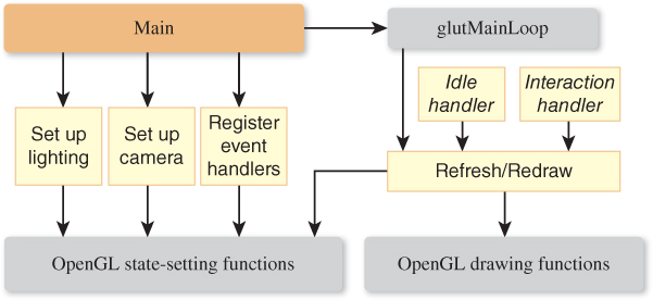
OpenGL library bindings are available for a large variety of languages, but in this discussion we’ll use C/C++ as our example language. Our program’s main() function uses GLUT to perform many of the initialization activities, starting with an obligatory call to glutInit:
1 int main( int argc, char** argv )
2 {
3 glutInit( &argc, argv ); // Boilerplate initialization
Next we request color support and depth buffering (also known as Z-buffering, used for hidden-surface removal as described in Chapter 36):
glutInitDisplayMode( GLUT_RGB | GLUT_DEPTH );
Then, we call a sequence of three GLUT functions to create the window that will be assigned to our application. The first two function calls allow us to specify the optimal initial size and position for the new window.
1 // Specify window position (from top corner)
2 glutInitWindowPosition( 50, 50 );
3 // Specify window size in pixels (width, height)
4 glutInitWindowSize( 640, 480 );
5 // Create window and specify its title
6 glutCreateWindow( "OpenGL Example" );
The result is a window whose client area (see Section 2.2) has the specified position and size. The application is free to further divide the client area into different regions; for example, to include user-interface controls. In the following call to glViewport, we reserve the entire client area for use as the 3D viewport:
1 glViewport(
2 /* lower-left corner of the viewport */ 0, 0,
3 /* width, height of the viewport */ 640, 480 );
OpenGL provides a variety of rendering effects, and with the function calls shown below, we specify that the front side of each triangle be filled using Gouraud’s smooth shading. (Alternatively, we can make the pipeline act as a point plotter or as a wireframe renderer, for example.)
1 // Specify Gouraud shading
2 glShadeModel( GL_SMOOTH );
3
4 // Specify solid (not wireframe) rendering
5 glPolygonMode( GL_FRONT, GL_FILL );
Initialization continues with calls to initialization routines that we will show later:
1 setupCamera();
2 setupLighting();
The main function is near its end, and still nothing has been drawn. It is time to register our application’s display handler to ensure GLUT will know how to trigger the generation of the initial image:
1 glutDisplayFunc(
2 drawEntireScene // the name of our display-event handler
3 );
The final act in the main function is the transfer of control to GLUT:
1 // Start the main loop.
2 // Pass control to GLUT for the remainder of execution.
3 glutMainLoop(); // This function call does not return!
4 }
Once GLUT has control, it will invoke the registered display function to trigger the generation of the program’s first rendered frame.
16.2.3. Lighting and Materials
OpenGL’s fixed-function lighting/materials model is somewhat different from that of WPF as described in Chapter 6, but any effect achievable in one system can effectively be emulated in the other quite readily. Because of this similarity, we omit this portion of the code, but the web materials for this chapter include it.
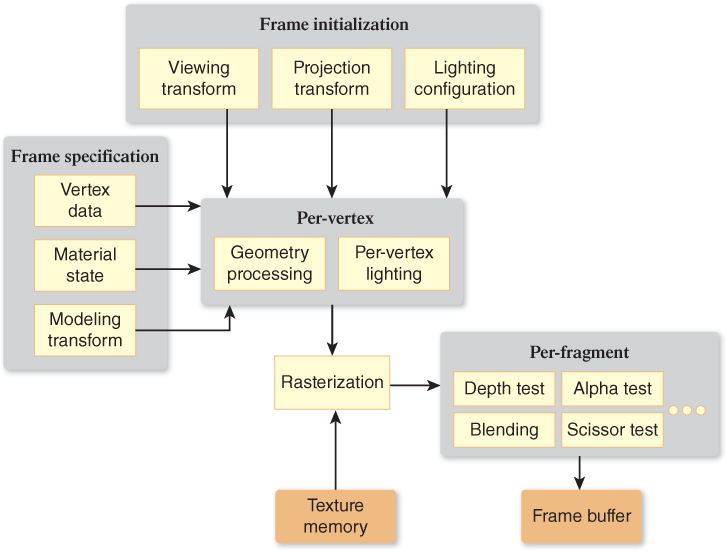
16.2.4. Geometry Processing
A simplified view3 of the OpenGL fixed-function rendering pipeline is shown in Figure 16.3; it might be useful to review Section 1.6.2 if some of the terms (e.g., “fragment”) are unfamiliar to you. In a fixed-function pipeline, the application’s focus is on configuring and feeding data to the per-vertex stage, as is exhibited by the locations of the two boxes representing application input and their varied contents toward the front of the pipeline. The rest of the pipeline, including rasterization and the many per-fragment operations at the end of the pipeline, use hardwired algorithms controlled via a number of configuration parameters.
3. This simplified view omits pixel data and operations such as bitmaps, images, texture setup, and direct framebuffer access.
As explained in Section 1.6, every 3D graphics system includes geometry processing that controls the conversion of geometric data (e.g., mesh vertices) successively from the modeling coordinate system (“object coordinates” in OpenGL nomenclature) to the world coordinate system, continuing on to the camera coordinate system (depicted in Figure 1.15, known in OpenGL as the “eye coordinate system” or “eye space”), and ultimately to some physical “device” coordinate system.
Coordinate-system transformations are performed via matrix arithmetic, as described in Chapters 7 and 11. Matrices are set up by the application using an abstraction provided by the immediate-mode API; we describe the OpenGL fixed-function abstraction below. Internally, the IM layer manipulates the matrices to prepare them for transmission to the GPU. The GPU itself may perform further manipulations to maximize the speed of computations and it must extend the pipeline’s scope further to produce physical/screen-pixel coordinates. Our discussion here focuses solely on the IM-level abstraction.
In fixed-function OpenGL, the geometry processing is performed by what is called the transformation pipeline, which has the stages depicted in Figure 16.4.
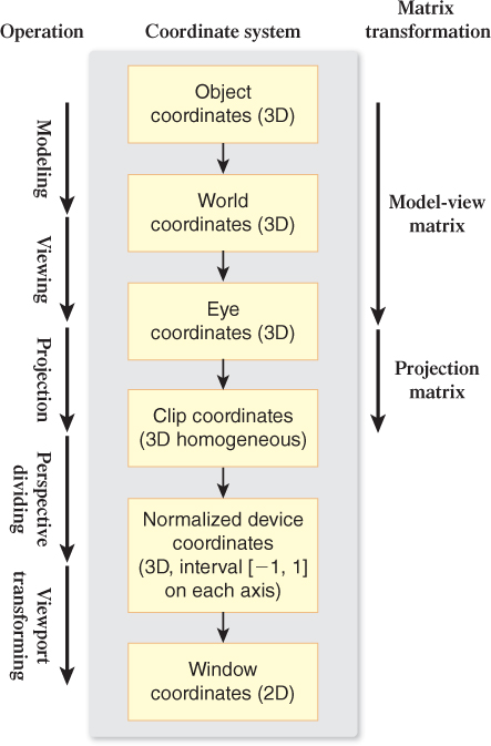
Figure 16.4: OpenGL’s geometry pipeline: a sequence of coordinate systems through which each 3D vertex of the original model progresses, via transformations, into its corresponding 2D display-device position.
The modeling stage brings the individual components’ coordinates from their original “raw” local coordinate systems into a single unified world coordinate system, and we examine how the modeling stage is used to implement hierarchical modeling in the online resources for Section 16.2.9. Then, the viewing stage transforms the coordinates into eye space, after which the camera is positioned at the origin and oriented in the canonical way described in Section 1.8.1.
Next, the projection stage works on normalizing the view volume’s shape and dimensions to OpenGL’s version of the standard perspective view volume described in Chapter 13, transforming the coordinates into 3D clip coordinates. The transformation pipeline includes two more stages that eventually yield the window coordinates that are sent to the rasterization module.
In OpenGL, the first three stages of the pipeline are controlled by the application via specification of two matrices, MMODELVIEW and MPROJECTION.
The MODELVIEW matrix handles the first two stages; the application has the responsibility of setting it (using utilities described in the next section) according to this equation:
MMODELVIEW = Mview · Mmodel
The order in which the two matrixes are combined ensures the modeling transform is performed on the incoming vertex (V) before the viewing transform is performed:
MMODELVIEW · V = Mview · Mmodel · V
The application separately sets (again using utilities described later) the PROJECTION matrix to define either a perspective or parallel view volume and its corresponding projection.
There is a good reason why OpenGL’s designers combined modeling and viewing, but kept projection separate. Typically, the camera view volume’s shape (defined by MPROJECTION) is quite static, persistent for an entire scene or even for the entire application’s lifetime. However, the camera’s location and orientation (Mview) is typically as dynamic, if not more so, than the scene objects themselves. By isolating the specification of camera shape/projection from the specification of camera position/orientation, OpenGL’s design makes it natural to specify these in different parts of the program structure/flow. Normally, setting the projection matrix will be more of an “initialization” operation, whereas specifying the viewing matrix is a part of each new animation frame’s computation, typically done just before scene construction commences.
16.2.5. Camera Setup
As described above, the camera specification is divided into two matrix specifications: viewing and projection.
To assist in specifying the latter, GLU provides the convenience function gluPerspective to compute the matrix for the common perspective-projection case of a symmetric frustum.
For example, to set the projection matrix (typically as part of an initialization sequence) to match the perspective camera we had specified in Section 6.2 for our pyramid scene, we perform this sequence:
1 // Prepare to specify the PROJECTION matrix.
2 glMatrixMode( GL_PROJECTION );
3
4 // Reset the PROJ matrix to ignore any previous value.
5 glLoadIdentity();
6
7 // Generate a perspective-proj matrix,
8 // append the result to the PROJ matrix.
9 gluPerspective( 45, // y-axis field of view
10 (640.0/480.0), // ratio of FOV(x) to FOV(y)
11 0.02, // distance to near clip plane
12 1000 );// distance to far clip plane
Note that each OpenGL or GLU matrix-calculation function performs two actions: (1) calculates the matrix that meets the specification given by the parameters, and (2) “appends” (via matrix multiplication) it to the current value of the matrix that is currently being specified. This is why the call to glLoadIdentity is important; without it, the calculated perspective matrix would be combined with, instead of replacing, the current value of the projection matrix.
Now, let’s set up the viewing transformation, typically one of the first operations in the preparation for rendering each frame of the animation. We describe the camera’s position and orientation using a GLU convenience function, providing parameters equivalent to those used for WPF camera specification:
1 // Prepare to specify the MODELVIEW matrix.
2 glMatrixMode( GL_MODELVIEW );
3 glLoadIdentity();
4
5 // Generate a viewing matrix and append result
6 // to the MODELVIEW matrix.
7 gluLookAt( 57,41,247, /* camera position in world coordinates */
8 0,0,0, /* the point at which camera is aimed */
9 0,1,0 ); /* the "up vector" */
16.2.6. Drawing Primitives
OpenGL provides several mesh-specification strategies, including the efficient triangle-strip and triangle-fan techniques described in Chapter 14.
The application is responsible for representing curved surfaces via tessellation into triangles; additionally, the application is expected to provide the vertex normal for each vertex. Since complex models are typically either computed via mathematics (in which case the normal is easily derived as part of that algorithm) or imported by loading a model (which often includes precomputed normal values), this requirement is rarely inconvenient.
The application can choose from several strategies for transmitting the mesh specification to the platform, including techniques for managing and using GPU hardware RAM (e.g., vertex buffers or VBOs, described in Section 15.7.2). In this example, for simplicity, we use the Compatibility Profile’s per-vertex function calls which are inefficient (and no longer present in the Core API) but popular in demos and “hello world” programs. To use this strategy as demonstrated in the code below, set the current material, initiate mesh-specification mode, enumerate each vertex one at a time (interleaved with control of the current-vertex-normal state variable), then end the specification mode. Let’s specify the same solid-yellow pyramid that we constructed in Section 6.2:
1 // Specify the material before specifying primitives.
2 GLfloat yellow[] = {1.0f, 1.0f, 0.0f, 1.0f};
3 glMaterialfv( GL_FRONT, GL_AMBIENT, yellow );
4 glMaterialfv( GL_FRONT, GL_DIFFUSE, yellow );
5
6 glBegin( GL_TRIANGLES );
7
8 The platform is now in a mode in which each trio of calls to
9 glVertex3f adds one triangle to the mesh.
10
11 // Set the current normal vector for the next three vertices.
12 // Send normalized (unit-length) normal vectors.
13 glNormal3f( ... );
14
15 // Specify the first face’s three vertices.
16 // Specify vertices of the front side of the face
17 // in counter-clockwise order, thus explicitly
18 // identifying which side is front versus back.
19 glVertex3f( 0.f, 75.f, 0.f );
20 glVertex3f( -50.f, 0.f, 50.f );
21 glVertex3f( 50.f, 0.f, 50.f );
22
23 // Set the current normal vector for the next three vertices
24 glNormal3f( ... );
25
26 glVertex3f( 0.f, 75.f, 0.f ); // Specify three vertices
27 glVertex3f( 50.f, 0.f, 50.f );
28 glVertex3f( 50.f, 0.f, -50.f );
29
30 ... and so on for the next two faces ...
31
32 glEnd(); // Exit the mesh-specification mode
33
34 The mesh is now queued for rendering.
16.2.7. Putting It All Together—Part 1: Static Frame
In contrast to WPF, which automatically updates the display to represent the current status of the scene graph, immediate-mode packages place the burden of display refresh on the application. First let’s look at a static-image generator, and then we’ll add dynamics.
Consider the case of a program that is to generate a single static image; in such a case, the rendering activity is only needed
• As part of initialization, to generate the first rendering
• Whenever the window manager reports to GLUT that the image has been damaged and needs repair (e.g., upon closing of a window that was partially covering the OpenGL window)
In this situation, the display function typically looks like this:
1 void drawEntireScene()
2 {
3 Set up projection transform, as shown above.
4 Set up viewing transform, as shown above.
5 Draw the scene, via an ordered sequence of actions, such as:
6 Set the material state.
7 Specify primitive.
8 ...
9
10 // Final action: force display of the newly-generated image
11 glFlush();
12 }
16.2.8. Putting It All Together—Part 2: Dynamics
Let’s extend the scenario to include dynamics; let’s have our simple pyramid model spin around the y-axis as though on an invisible turntable, the visualization technique used in the lab software for Chapter 6 to demonstrate the effect of directional lighting.
In an object-oriented system, each node in the hierarchical scene specification supports attached transformation properties, so you would perform this animation by attaching a rotation transformation to the pyramid primitive and tasking an Animator element to dynamically modify the amount of rotation. This technique is identical to the clock-rotation technique we used in Chapter 2.
In an immediate-mode platform, we perform modeling by direct manipulation of the MODELVIEW matrix. We’ve already learned how to initialize the MODELVIEW matrix with the viewing transform. To achieve the spinning dynamics, we must change our scene-generation function slightly, by appending a rotation transformation to the MODELVIEW matrix just before drawing the scene.
We elaborate on this technique, and provide source-code examples, in the online material for this chapter.
16.2.9. Hierarchical Modeling
Previously, we presented two examples of hierarchical modeling: a 2D clock in Chapter 2, and a 3D camel in Section 6.6. In those examples, we learned how to create a scene using a retained-mode platform such as WPF: The application sets up the scene by creating a hierarchy of component nodes (attaching instance transforms to specify initial placement), and animates the scene by adjusting the values of the joint transformations attached to the nodes. This is an intuitive way to work, since the scene graph’s structure exactly mirrors the physical structure of the scene being modeled.
Now, reconsider the camel hierarchy shown in Figure 6.41. How can we construct this model using an immediate-mode platform?
The challenges here are twofold.
• The IM platform has no facility for storing the model. The application is wholly responsible for representing the model’s hierarchy, and for computing and storing the values of all transforms that control position and orientation.
• Section 10.11 describes the graph-traversal and matrix-stack techniques necessary to compute the composite transformation matrix to properly position and orient a particular leaf component in the hierarchy. A retained-mode platform performs this calculation automatically, but this burden rests on the application when using an IM platform.
To satisfy the need for model representation,4 there are two approaches.
4. Here, we are concerned with a model that has only the geometric data necessary to generate the target image, but the focus of a typical real-world application is an “application model” (see Section 16.4) that encapsulates many different data types, graphical and nongraphical.
• Create a custom scene-graph module, duplicating functionality found in a typical RM layer (see Section 16.4), in terms of both storage (such as a hierarchical component graph, and a database of transform values) and processing (traversal and generation of the IM instructions).
• Use the program’s call-graph hierarchy to represent the model’s structure, by writing a distinct function for each type of node (grouping or primitive), with the functions for higher-level nodes calling the functions for lower-level ones.
In the online resources for this chapter, we examine the latter approach in detail, including source code for a complete working example.
16.2.10. Pick Correlation
One of the advantages of an RM platform is its support for pick correlation, the determination of the primitive that is the target of a user-initiated mouse click or other equivalent device action. For example, WPF converts a given 2D viewport pick point’s coordinates into a pick path that identifies the entire path from the root of the scene graph down to the leaf primitive.
Of course, an IM platform cannot automate such functionality since it does not retain the scene. Thus, an IM application often uses custom correlation logic, running an algorithm such as ray casting (Chapter 15) while traversing through the application’s scene data store. OpenGL offers an alternative technique that uses the name stack to efficiently automate hierarchical pick correlation. This technique is described in the online materials for this chapter.
16.3. The Programmer’s Model: OpenGL Programmable Pipeline
At its core, real-time graphics is still done using lights, meshes, materials, transformations for viewing and modeling, etc. The progression from fixed-function to programmable has not changed its essence. But where these types of objects reside in the application source code has shifted to programs written in shader languages and installed in the GPU, as described in detail in Chapter 33.
16.3.1. Abstract View of a Programmable Pipeline
Let’s examine an abstract view of a programmable pipeline, shown in Figure 16.5 and explained in the next few paragraphs. To keep this model simple, we omit texture data/operations, show only vertex and fragment shaders, and omit feedback loops. We use OpenGL terminology, but this is also applicable to Direct3D.

If this diagram seems to be a bit incomplete, you’re on the right track! Where are the lights, materials, and camera? They are all present, but only “in spirit”: in the empty input-related yellow boxes and in the two shader boxes. Whereas the fixed-function pipeline can be considered a configurable appliance, the programmable pipeline is a computer on which you install an application of your own construction. Let’s first examine the pipeline’s semantics in the absence of a particular application, and then we’ll look at how this pipeline might appear when loaded with an actual program.
The application sends batches of vertices through this pipeline, each batch representing a mesh for which certain characteristics (e.g., material or lighting) are constant across its vertices. The vertex shader is a function that is called once for each vertex in the batch, receiving as input the vertex and associated attributes such as the vertex normal or the texture coordinate. The vertex shader also has access to any number of per-batch “uniform” inputs providing information that is constant for the entire batch (e.g., camera characteristics).
What the vertex shader does is up to the programmer. At the least, its output must include the vertex transformed to clip coordinates (i.e., already passed through modeling, viewing, and projection transformations), but it also may include any amount of other output data values to “tag along” with this vertex to the next stage of the pipeline. Typically, a calculated vertex color is one of the outputs, but there is no limit to the number of outputs or their semantics. Each output is typically marked as “smooth,” which tells the rasterizer stage in the pipeline to interpolate that particular output’s values for the pixels that lie between the vertices. (The alternative is “flat,” which disables this interpolation.)
What lies between the vertex and fragment shaders is a mini-pipeline of several modules,5 shown in Figure 16.5 as a single box. They work together to complete the transformation pipeline to convert to window coordinates, to perform clipping/culling against the view frustum, and to perform rasterization to produce a sequence of output fragments.
5. On some hardware platforms, this part of the pipeline is also programmable, through use of a third type of shader, known as a “geometry shader.”
The fragment shader (whose equivalent in Direct3D is called the “pixel shader”) is called once for each fragment and receives the fragment’s location (in window coordinates) and the already-interpolated varying outputs from the vertex shader. In very simple cases, the fragment shader often does nothing but pass the color unchanged through to the next stage, but the fragment shader is essential for lighting algorithms for which simple linear interpolation between vertices is insufficient, and is also instrumental in special effects such as blurring.
At the end of the pipeline lie the per-fragment operations, similar to those found in the OpenGL FF pipeline.
16.3.2. The Nature of the Core API
The OpenGL Core API retains only a fraction of the entry points that were present to support the FF pipeline. The techniques for specifying and transmitting textures and meshes have not changed significantly, and end-of-pipeline activities like blending and double-buffering are similar. However, all other information and operations now lie inside in the uniforms, attributes, and shader code. The leaner OpenGL Core API is mostly concerned with activities of the following types:
• Buffer object management—control over all data stored on the GPU, including allocation/deallocation and data transmission
• Drawing commands—sending meshes down the pipeline
• Shader-program management—downloading, compiling, activating, and setting up uniforms and attributes
• Texturing management—installation and management of texture data structures for use by vertex and fragment shaders
• Per-fragment operations—control over per-fragment operations at the end of the pipeline, such as blending and dithering
• And framebuffer direct access—pixel-level read/write access
16.4. Architectures of Graphics Applications
We now discuss the general structure of a typical graphics application, some approaches to speed up certain parts of this structure, and various kinds of software designed to offload that work from the typical designer.
16.4.1. The Application Model
A typical 3D application includes an application model (AM)—a collection of data, resident in a database or in data structures, whose application-domain semantics go beyond a mere rendered image, but for which an image is one possible view of the AM.
In our simple WPF-2D clock application, the AM contained only the current time of day, but it could be extended to include alarm-related data (date, choice of alarm sound, enabling of “snooze control,” etc.) or support for multiple time zones. Note that the AM need not include any inherent geometry; for example, there’s nothing geometric about the time of day, and the rotation-based analog display of clock time is simply one way to display that data.
Most applications have a heterogeneous AM containing both nongeometric and geometric data, and the latter can be further subdivided into abstract geometric (not in a form ready for the IM layer) versus ready for rendering (in a form ready for the IM layer, e.g., geometry in the form of a triangle mesh).
Consider the breakdown of the AM of a chess application.
• Nongeometric data would include
– Current board location of each piece (i.e., the square on which it resides)
– Record of each move since the game started, to facilitate export of a game “transcript”
– Chess strategy data used by the game to plan its moves
– Duration of the game in progress, the player whose turn it is, the amount of time left for her move, etc.
• Abstract geometric data might include
– Mathematically defined shapes of the pieces (which must be converted into meshes in order to be made ready for rendering)
– Motion paths, specified as cubic Bézier curves, to support animation of the movement of pieces from square to square
• The ready-for-IM geometric data might include
– Geometry and materials for rendering the chessboard itself
– Camera definitions for several points of view (if the UI allows the user to choose from several POVs, e.g., directly overhead, POV from seated avatar, etc.)
– Modeling transforms for the pieces (e.g., if the user is able to control the 3D positions and orientations of the pieces beyond their abstract locations on specific squares)
Now consider the highly complex AM for a CAD/CAM representation of a jet airliner, consisting of millions of components, each including geometric, spatial layout, and connectivity/joint data; behavioral data used in aircraft-operation simulation; part numbers, costs, and supplier IDs used in procurement; maintenance/repair instructions or cautions; and much more. In addition, each component “lives” in several organizational systems for the purpose of searching and filtering; for example, a spatial organizational system might separate components into regions (e.g., cockpit, main cabin), but a functional one might separate components into distinct systems such as electrical or hydraulic.
These databases thus act as a confluence of many types of data, used and manipulated by a large variety of different systems and applications, of which only a fraction are “computer graphics” programs.
For the purposes of this text, we are concerned only with the data that is either intrinsically geometric, or can be represented geometrically for the purpose of rendering.
16.4.2. The Application-Model-to-IM-Platform Pipeline (AMIP)
We now consider how an IM-based application drives an IM platform, which in turn drives the GPU. Every such graphics application must implement—in addition to its own special semantics/logic—a multistage process that we call the “Application-Model-to-IM-Platform pipeline,” or AMIP. The AMIP is the front part of the client (CPU) side of the complete rendering pipeline depicted conceptually as a sequence of stages, each executing a designated task, in Figure 16.6.
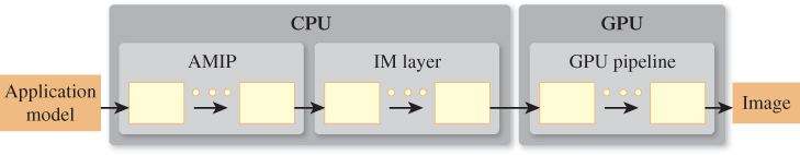
Figure 16.6: Abstract view of the typical application pipeline transforming the application model into a scene delivered to the immediate-mode platform for rendering.
At its most basic, the AMIP is composed of a traversal of the AM to do the following.
• Determine the scene to be rendered, including all geometry, materials, lighting/special effects, and camera configuration. The application traverses the application model to extract the data relevant to the scene, transforming any nongeometric data into a geometric representation for inclusion in the scene. This is analogous to the act of generating a view of a database, an action requiring both selection (extraction based on query criteria) and transformation (arbitrary computation on or reformatting of extracted data fields).
• Calculate the sequence of API calls needed to drive the IM layer to produce the image of the scene.
Figure 16.6 depicts the complete rendering pipeline from a functional point of view. Another way to describe a graphics application is from a software-engineering point of view: enumerating the layered software stack of components, with the custom application code at the top of the stack, the graphics hardware driver at the bottom, and intermediate platforms/libraries in between.
The graphics-related stack for a typical 3D graphics application is made up of at least three layers (see Figure 16.7), and may contain four layers (see Figure 16.8) if a retained-mode middleware platform is used to assist with AMIP duties.
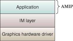
Figure 16.7: Software stack for an application that describes the scene directly to the immediate-mode platform.
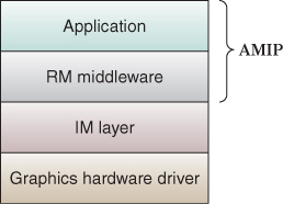
Figure 16.8: Software stack for an application that constructs the scene using retained-mode middleware.
How the AMIP’s tasks are sequenced within the pipeline and divided between layers of the software stack is volatile, as technologies evolve; moreover, AMIP tasks that currently typically live on the CPU side are subject to movement to the graphics hardware as GPU programmability becomes more exploited. We will address this “division of labor” later; first let’s focus on the kinds of tasks present in the AMIP.
In all but the most trivial applications, it is necessary for the AMIP to work in a highly optimized way in order to ensure scalability—that is, to ensure adequate performance (especially for real-time animation) even as the size and complexity of the scene grows. The term “Large-Model Visualization” (often abbreviated LMV) is typically used to describe applications or platforms that handle scenes of extremely high complexity such as a CAD model of a jetliner or cruise ship.
The primary goal of the AMIP’s optimization tasks is to reduce consumption of resources such as the following:
• Bandwidth between the CPU and the GPU, by minimizing data transmission to the GPU
• GPU memory consumption, for example by reducing the size of geometry data cached on the GPU
• And GPU processing cycles, by generating an efficient sequence of IM-layer instructions to the GPU to render the scene
CPU-side resources are used to perform these optimization tasks, so there is a tradeoff here: The benefit of the reduced consumption later in the pipeline (especially regarding the GPU) comes at the cost of extra work being done earlier in the pipeline.
In general, the AMIP is composed of stages through which scene data flows. These stages operate sequentially, or partially in parallel, performing optimization duties in three categories:
1. Reducing scene complexity
2. Generating an efficient stream of instructions to the IM layer
3. And avoiding redundant computation activities through appropriate caching
16.4.2.1. Reducing Scene Complexity
There are three categories of tasks that help reduce the amount of graphical data sent to and processed by the underlying IM layer, which we now describe.
16.4.2.1(a). Extracting the Scene from the “Universe”
In large applications, the application model may contain or represent a “universe” of graphical objects that are not necessarily all visible simultaneously. The AMIP thus extracts the relevant subset of the universe, based on application data that specifies the desired rendering goals. For example, in an airplane CAD application, the universe is the entire airplane’s specification, and the subset to be rendered might be determined by the user’s selection of the subsystems (such as electrical, HVAC, or hydraulic) of current interest.
As another example, consider a multilevel game, in which each level is a completely different subworld—the application need only extract the current subworld to determine the scene to be rendered.
16.4.2.1(b). Reducing the Scene to the Minimal Potentially Visible Set of Primitives
The AMIP’s focus here is on high-level culling—elimination of entire primitives or (better yet) large portions of the scene that need not be rendered. This is in contrast to hidden-surface removal activities performed by the GPU—such as back-face culling as described in Section 36.6, or occlusion culling on a per-pixel level through the depth buffer as described in Section 36.3.
Together, the high-level (CPU-side) and low-level (GPU-side) culling activities work together toward a common goal of reducing scene complexity and thus GPU workload.
It is tempting to think of pre-GPU culling as unnecessary, that as GPUs become more powerful and bandwidth increases, there is less justification for throwing CPU resources at the problem of determining the potentially visible set. However, the GPU-side visible surface determination has a cost that is linear in the number of primitives. Thus, when one considers a Boeing 777 model—which has more than 100,000 unique parts and several million fastener parts—it becomes obvious that there continues to be a need for optimizing the sequence of commands and data sent to the hardware rendering pipeline.
Below is an unordered list of modules of this category, many of which require spatial data structures as discussed below in point 3(b):
View-Frustum Culling: As explained in Chapter 13, the camera’s location and viewing parameters determine the geometry of the view frustum, and only geometry lying inside the frustum is visible. This culling stage seeks to identify and eliminate portions of the scene that lie wholly outside the frustum. Implementation is typically performed via arrangement of the scene’s contents in a Bounding Volume Hierarchy (BVH), as described in Section 36.7; however, other data structures (e.g., BSP trees discussed in Section 36.2.1) have been used for certain situations (e.g., static scenes).
Sector-Based Culling: In many applications, the scene’s environment is architectural, that is, located in the interior of a building, with walls segmenting space into “sectors” and windows/doors creating “portals” that connect adjacent sectors. A number of algorithms, described in Section 36.8 and sometimes called portal culling techniques, are available to cull objects in these kinds of environments.
Occlusion Culling: Consider a scene modeling midtown Manhattan, seen from the point of view of a pedestrian at just one intersection. If the depth of the view frustum covers many city blocks, each visible surface, especially those close to the viewer, is occluding a very large number of objects. In these types of environments, there can be great advantage in removing these occluded objects.
Contribution Culling/Detail Culling: A visible primitive, or an entire sub-portion of the scene, may be too small and/or too far away to make an impact on the rendering. This culling step is designed to detect and dismiss such content. Some applications might choose to use this type of culling only when the viewer is in motion, since the absence of small objects will very likely go unnoticed during dynamics but may be detectable when the camera is at rest.
16.4.2.1(c). Reducing the Transmission/Rendering Cost of Geometric Shapes
In this set of activities, complex geometric shapes specified via meshes either are encoded to reduce the GPU-side rendering cost or the size of the data buffers needed to transfer the specification to the GPU, or are simplified by reducing the mesh’s complexity (e.g., reducing the number of triangles and vertices).
Reencoding is the act of converting the mesh’s specification to one that is more quickly processed by the graphics hardware. For example, converting to triangle strips [EMX02] is common since many hardware pipelines are highly optimized for that succinct encoding type.
Simplification is a form of compression similar to the image compression of JPEG or audio compression of MP3. The compression is lossy in that the resultant geometry is not as accurate as the original. But just as MP3 compression produces music files that are “good enough” for many purposes, geometric simplification also can be tuned to be satisfactory for specific applications.
For example, if an object or the viewpoint is in motion, it may be possible to simplify the object without the viewer being aware. Or, if the object’s “importance” (measured in terms of how many pixels its projected image takes up on the viewport) is lower than some threshold, a certain amount of simplification may be possible without damage to the object’s legibility.
There are numerous types of geometric simplification, including the following.
• Continuous Level of Detail / Multiresolution Geometry / Geomorphing / Selective Refinement/Progressive Meshes/Hierarchical Dynamic Simplification
A number of algorithms, known by a variety of names, can be used for automatic simplification of a mesh in a manner that fine-tunes the amount of simplification based on the importance (as described above) of the object’s image. These algorithms vary widely in their strategies and usage scenarios, and they should be studied by any developer needing “just enough but not too much” simplification.
As an example, a progressive mesh (described in detail in Section 25.4.1) provides for storage of a mesh at many resolutions in a single data structure. The structure can be thought of as a sequence: The coarsest (least-expensive, lowest-quality) mesh is stored as the “core,” followed by a sequence of “reconstruction records” describing how to incrementally restore the higher-resolution information. The renderer of this mesh sequence can choose to stop reconstruction at any point in the sequence; the more the processor continues to execute the reconstruction records, the closer the resultant mesh is to the original resolution.
Note that opportunities for implementation of some of these algorithms lie both in the AMIP and directly on the graphics hardware.
• Discrete Level of Detail
When the application needs full control over the simplified geometry, this technique can be used instead of fully automated mesh simplification. Key objects are specified via multiple mesh definitions (e.g., high-, medium-, and low-detail versions), and the application uses the one appropriate for the object’s current importance (as described above).
• Simulating Complex Geometry
For certain applications (e.g., the bumpy surface of an orange, or rocky terrain seen from afar), instead of representing the geometry in the actual mesh and bearing the cost of lighting/shading calculation, an application can use tricks to fool the eye into seeing complex geometry that is not actually part of the mesh. Texture mapping, as described in Section 1.6.1, is a primitive technique that wraps the mesh with an image in order to provide color and translucency variation. More sophisticated algorithms, described in Chapter 20, include normal mapping, displacement mapping, bump mapping, and procedural texturing. As an extreme case of cost reduction, consider the “billboard” technique described in Section 14.6.2, in which far-away complexity is simulated via a texture-mapped planar polygon.
• Subdivision Surfaces / GPU Tessellation
In contrast to simplification techniques, this technique has the opposite goal—it uses an iterative subdivision algorithm (see Section 14.5.3 and Chapters 22 and 23) to add complexity to a coarse “base mesh” to provide a smoother appearance. This is an optimization technique due to its use of the GPU to perform the tessellation; the CPU side deals only with the coarse base mesh, thus reducing use of CPU/GPU bandwidth. Since the process is iterative, the GPU-based tessellation can adjust the amount of smoothing work based on the primitive’s distance from the viewer, thus providing a kind of variable level-of-detail control.
16.4.2.2. Generating an Efficient Sequence of IM-Layer Instructions to Render the Simplified Scene
The graphics hardware pipeline is a complex combination of functional units, and achieving maximum throughput requires expert knowledge of the pipeline’s idiosyncrasies and potential bottlenecks. Certain types of operation sequences can cause “pipeline stalls” that radically undermine performance. As the pipeline has adapted to relieve these bottlenecks over the years, new bottlenecks have arisen, presenting opportunities for further adaptation.
In particular, state changes (e.g., a change in the current-material state variable, or a switch to a different vertex shader) disrupt pipeline throughput and should be minimized by careful ordering of the primitive-drawing sequence. The actual cost varies by API, hardware platform, driver software, and type of state variable being modified. Nevertheless, as a rule, each state change should be followed by the generation of as many primitives as possible; thus, as part of the AMIP, logic should analyze the potentially visible set for the purpose of reordering the primitives so as to draw in a batch all primitives that require the same state configuration. In a chess application, one might model all the black pieces as obsidian and the white pieces as onyx. It then makes sense to render all the black pieces before all the white ones, or vice versa.
The modification of specification order generally does not have an impact on the final rendered image, but it should be noted that the use of translucent materials presents an exception and does complicate this optimization task (and others, e.g., occlusion culling).
16.4.2.3. Using Caching to Avoid Redundant Computations in Performance of Tasks in Categories 1 and 2
The CPU and memory resources necessary to perform the activities described above for task categories 16.4.2.1(a–c) and 16.4.2.2 can be substantial. But many of these activities, when executed to produce frame i, produce results that remain useful for frame i+1, if the difference between the two frames meets certain requirements. Thus, caching is of value in reducing the CPU cost of such activities.
Caches used for this purpose are called acceleration data structures and are used in two distinct ways.
• Cache the result of computations.
– For example, consider 16.4.2.2. The generated IM-layer instruction sequence associated with static portions of the scene can be cached and reused in successive frames; moreover, this cache can even be downloaded to the graphics hardware as a display list to eliminate its being redundantly sent across the CPU/GPU boundary.
– As another example, consider 16.4.2.1(b). Simplified meshes computed through algorithms such as those listed above should also be cached, and, here again, there is the opportunity for either client-side (CPU) or server-side (GPU) storage.
• Cache the data that is used in the performance of these computations.
– For example, consider 16.4.2.1(a). View-frustum culling is typically performed by organizing the candidate primitives into a BVH (see Chapter 37), cached and reused across frames; moreover, the longevity of this cached data structure can be extended by ensuring that it is selectively updated as needed when changes are made to the scene’s geometry.
– As another example, consider 16.4.2.1(b). The decision-making logic for the various types of conditional simplification is typically performed through computation of the cost (a measurement of the geometry’s complexity and thus of the cost associated with rendering it) and value (a measurement of how much screen real estate its image will take up) for each graphics object. The value:cost ratio is then used by the algorithm that determines how much simplification of a particular object is tolerable. The value/cost information can be cached, of course, keeping in mind that the “value” parts of the cache will need to be invalidated as POV changes occur.
The software that maintains an acceleration data structure is often nontrivial in design; we address this topic further in Section 16.4.3.
As you were reading the above list of common AMIP tasks, you may have been creating a mental image of a well-defined sequential pipeline such as that shown in Figure 16.9.
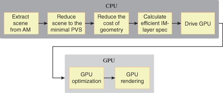
It’s important to note again that this is a highly conceptual view of the complete AM-to-rendered-image graphics pipeline. Real-world implementations vary from this abstract view in several ways.
• The tasks are not necessarily sequential; the use of parallel computation may be possible for some tasks.
• The order in which we show these tasks is conceptual and not necessarily adhered to by actual software/hardware.
• Some types of tasks may be split across several software/hardware modules, and (for extremely high scalability) across multiple CPUs and GPUs.
• We’ve not discussed GPU internals here; consult Chapter 38 for a discussion of modern graphics hardware.
With this in mind, let’s next turn our attention to the CPU-side software stack, in particular the four-level stack, which includes a retained-mode middleware layer designed to handle a large proportion of the AMIP’s duties.
16.4.3. Scene-Graph Middleware
You have now been introduced to two abstraction levels for 3D graphics specification: immediate mode (IM) and the higher-level retained mode (RM). You already know that two key responsibilities of the RM layer are to provide for storage of a scene graph, and to provide functionality to traverse the scene graph to generate the instructions to be sent to the IM layer to produce the image.
Additionally, in Section 16.2.9, we noted that an application built directly atop the IM layer typically necessarily contains custom-built modules duplicating basic RM functionality, simply because scene storage (and converting such into an image) is so commonly needed in graphics applications.
Let’s take a more complete look at the functionality of RM middleware. An RM-based application extracts information from the application model, and uses the RM API to construct the scene graph that resides in the middleware layer. Some of the programmer conveniences gained by the middleware’s maintenance of the scene description include
• Object-oriented representation of key 3D graphics concepts (primitives, transforms, materials, textures, camera, lights), providing programmers with an intuitive API for setting up scenes
• Support for hierarchical modeling
• Support for dynamics through incremental editing of the scene description
• Support for hierarchical pick correlation
These conveniences are found in virtually all RM middleware; however, in addition to these features, RM middleware designed for optimal performance optionally can perform any of the post-application-model AMIP optimization tasks listed in Section 16.4.2, as shown in Figure 16.10. Many RM layers perform very little optimization, some are designed for optimal scalability and performance, and some are simply conveniences offering no optimization at all. (For specifics, visit the online materials for this chapter, which contain a curated list of scene-graph platforms.)
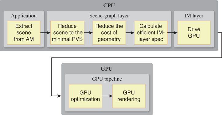
Figure 16.10: Sample distribution of AMIP responsibilities in an application using retained-mode middleware.
16.4.3.1. Optimization via Acceleration Data Structures
To achieve performance gains, some RM implementations build acceleration data structures (described in Section 16.4.2.3) to store information useful for optimization. Designing the software logic that maintains these data structures—illustrated in Figure 16.11 and covered throughout Chapters 36 and 37—is a nontrivial task, because the structures must be maintained as the scene graph is modified, requiring sophisticated logic to avoid unnecessary invalidations (i.e., premature discarding) of cached information, and to avoid the expense of wholesale regeneration of the structures.
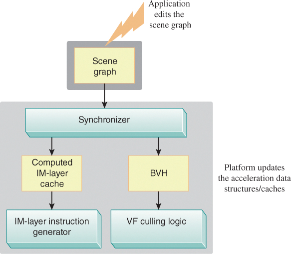
Figure 16.11: Abstract depiction of an RM layer providing two types of optimization discussed in Section 16.4.2 (view-frustum culling and IM-instruction reuse), showing the synchronization logic that ensures the acceleration data structures (BVH and IM-instruction cache, in this example) are updated when the scene graph is modified.
In addition to the CPU time allocated to maintaining these structures, there is also a nontrivial CPU memory cost as well. At the end of this section, we’ll visit the issue of the runtime cost of scene-graph middleware and discuss the cost/benefit tradeoffs.
16.4.3.2. Optimization of Static Scene Portions
An initially counterintuitive but then “obvious” maxim about scene graphs, proffered by Henry Sowizral, the designer of Java3D (a pioneering RM platform in terms of optimization support), is simply: Traversal of a scene graph is expensive and should be avoided to the fullest possible extent.
In particular, during real-time animation sequences, it is untenable for the scene graph to be retraversed for each individual frame of the animation. A scalable scene-graph platform thus minimizes traversal by performing tasks of the type mentioned in Section 16.4.2.3:
• Identifying—either automatically or via application-provided “hints” such as those in Java3D—graph nodes with static content
• Generating and caching acceleration structures for such “subgraphs”
• And not allowing dynamic components in the scene to affect these cached acceleration structures (which would lead to a high frequency of unnecessary cache invalidations)
When using an RM layer, you can assist the middleware with this task by isolating static from dynamic components in the scene graph. For example, if the root node’s first child is a node X containing all static parts of the scene, the subgraph rooted by X need be traversed only once, and that traversal will prepare the acceleration data structures that provide for efficient generation of that part of the scene. The remaining children of the root would be marked as dynamic and not allowed to alter the acceleration structures for the static portion of the scene.
In an application that allows the viewer to travel through a static scene the entire scene graph can be handled in this way—that is, traversed exactly once to set up the acceleration structures that will efficiently generate each frame of the animation.
It is interesting to note that the generation and caching of the acceleration structures often involves “flattening” the scene-graph hierarchy, to eliminate traversal dependencies. Why? Well, remember Sowizral’s admonition: Avoid traversal! The goal of the acceleration structures is to give the optimization algorithms rapid access to ready-to-use data needed for their operation; to require the optimization logic to traverse the scene-graph hierarchy in order to interpret the acceleration data would be a serious slowdown.
16.4.3.3. Costs and Disadvantages of Retained-Mode Middleware
The benefits provided by an RM layer come at a cost. Development-related costs include the learning curve associated with the package’s API, and the time needed to gain the experience required to efficiently diagnose and repair bugs during development. (Of course, there is also a financial cost for commercial middleware products.)
Runtime costs include both CPU-side memory and processor usage, primarily in these two categories.
1. The scene graph itself is stored on the CPU side and its memory requirements can be nontrivial for highly complex scenes. Moreover, if the AM is predominantly geometric itself, the scene graph might be considered quite redundant with the AM.
2. The acceleration structures/caches used internally by the middleware’s optimization modules use CPU-side memory and can be nontrivial in size for highly complex scenes.
It is interesting to reexamine our camel-modeling application, and compare our OpenGL function-based approach with a scene-graph approach such as that presented in Chapter 6. Consider a desert scene with 100 camels moving as a caravan. What are the CPU-side memory requirements for each of these strategies?
In Section 6.6.4, we showed how reuse of the composite components at different levels of the hierarchy affected the number of nodes in the scene graph. We saw that component reuse resulted in resource savings at the cost of loss of detail in the animation control. Ultimately, if our target animation quality requires individual control over every joint in the scene, reuse of composite components is not possible and the cost of the scene-graph storage is at its highest. (Of course, the mesh data associated with the atomic components can be shared without any loss of control over joint animation.)
By contrast, it would at first glance appear that the function-based approach of Section 16.2.9 is highly scalable. The cost of the representation of the hierarchy’s design is indeed constant, since it lives in the compiled executable and is unrelated to camel count. Indeed, if the goal was to render 100 camels in random locations for a still-frame rendering, one could write a program calling the Camel() function 100 times with random nonretained instance and joint transforms. The CPU RAM cost would be truly a constant, unrelated to camel count. However, if animation of the caravan is required, at the very least the application model must include per-camel location/orientation status. And if complete control over each joint is required for high-quality animation, this AM-resident storage of camel information (with location, orientation, and status at all joints) starts looking more and more like a scene graph. The higher the requirement for control over the scene’s details, the more the AM will start having many of the qualities of scene graph, and the more time the development team will spend building what is essentially a custom scene graph and custom AMIP.
A development team choosing between constructing a custom AMIP and using a middleware platform to offload a lot of responsibility should take these costs into account. As noted, some of the costs (e.g., acceleration data structures) are unavoidable; however, a custom AMIP does offer the possibility of avoiding duplication of AM data. The redundancy of a middleware-resident copy of AM data, and its CPU-side cost in terms of both memory and processing cycles, is seen by many as a fundamental problem with general-purpose, domain-independent scene-graph middleware technology.
Yet, the conveniences of a hierarchical scene-graph and the automation of AMIP optimization are highly beneficial, and thus a more efficient platform architecture (described in the next section), which merges the AM and scene-graph data, has become popular in some specialized domains.
16.4.4. Graphics Application Platforms
In a few key application domains with large developer communities, the need for the convenience and optimizations of a scene-description database, coupled with the need for solutions to other problems common to that domain, have led to the development of what we call graphics application platforms.
The most prominent domain of this kind is game development. Consider the list of tasks associated with producing a 3D interactive game:
• Highly optimized AMIP
• Statistics/history recording/“score keeping”
• Audio (background music, synchronized sound effects)
• Physics for realistic dynamics
• Networking (for multiplayer games, LAN-based or Internet-based)
• Artificial Intelligence (for character/object autonomous behavior)
• Input-device handling
To provide a feature-rich foundation for game development, a number of game application platforms (often called game engines) have been made available as commercial products or open source projects. Many have evolved as a side effect of a team’s creation of a specific game product or series. Internal to the runtime module of a game application platform is a set of databases that can together be considered a “super scene graph” that stores the scene information interleaved with the application model. For example, in an auto racing game, a template representing an instantiable car might contain not only the expected geometric information (e.g., a scene-graph template representing the car’s geometry and appearance), but also its maneuverability characteristics (e.g., acceleration limitations, handling characteristics in sharp turns, etc.). Moreover, an instance of that template, representing an actual car involved in an ongoing race, would carry additional game-related information (e.g., current velocity, current angular momentum) in addition to the geometric current-location/orientation information that would be present in a normal scene graph.
Game development involves much more than just implementing the executable runtime, and thus mature game-development systems also often include utilities/IDEs that assist in design-time activities. For example, the popular Unreal game-development environment includes tools for the following:
• Three-dimensional model construction/editing, including facilities for loading existing models from a variety of file formats
• Character skinning/rigging for designing humanoid/animal figures that move realistically
• Art direction, including background painting, material design, and lighting design
Of course, graphics application platforms are available in other disciplines as well. For example, in the CAD/CAM domain, Autodesk’s AutoCAD system has evolved from an application to a platform with a high amount of configurability, a “super scene graph” database, and a rich API. Instead of trying a one-size-fits-all approach, AutoCAD offers distinct environments with targeted AM semantics for several subdisciplines, such as mechanical, architecture, factory-floor layout, etc.
16.5. 3D on Other Platforms
The computational requirements of 3D applications have in the past kept them as standalone applications running on desktop/laptop PCs or on specialized gaming platforms such as Xbox 360, PlayStation, Wii, etc. However, progress in both hardware capacity and software development is poised to increase the viability and use of “embedded” 3D.
16.5.1. 3D on Mobile Devices
The typical high-end smartphone or tablet includes a hardware-accelerated, programmable pipeline that includes vertex and pixel shaders. To provide a consistent hardware-independent API for these devices, a lightweight version of the OpenGL API has been developed, named OpenGL ES (Embedded Systems). This API is currently pervasive in the mobile space, with the notable exception of Windows-based phones and tablets driven via DirectX 9 APIs.
The design of the ES variant primarily involved adjusting to the limitations of mobile devices with regard to processing capability, memory availability, memory bandwidth, battery life, etc. For example, precision qualifiers were added to the shading language to allow applications to choose lower numeric precision to reduce use of the processor. Some features that place a large burden on the processor, such as pseudorandom noise computation, were eliminated. Additionally, the ES variant promotes the strategy of downloading precompiled (binary) shaders, since compilation of shader code is computationally expensive.
16.5.2. 3D in Browsers
Efforts to define a text-file format for 3D scene specification, suitable for Internet delivery of 3D content to web browsers (as well as for cross-application transfer of scene/model specifications), date back to 1994’s first version of VRML (Virtual Reality Modeling Language). Now extensively evolved and renamed X3D, this ISO standard maintained by the Web3D Consortium provides XML declarative specification of 3D scene graphs, supporting the fixed-function pipeline and shader extensions. Special scripting and interaction/animation nodes provide some dynamics, and navigation nodes provide for setting up walkthrough/flythrough navigation, making it more than just a generator of static images. However, the lack of native support for X3D in popular web browsers has slowed adoption, and the format has not gained traction with website authors outside of academia.
The potential for widespread use of 3D content on websites is far higher with WebGL, a JavaScript API native to most prominent browser brands, supporting immediate-mode 3D rendering into the HTML5 canvas. Based on OpenGL ES, it has no fixed-function pipeline and requires the use of shaders for all appearance control. Thus, programmers wanting a fixed-function model and/or a retained-mode scene graph will rely on middleware platforms, of which several are currently in development.
For information on this rapidly evolving topic, access the online materials for this chapter.
16.6. Discussion
This chapter has provided a brief introduction to graphics platforms with differing design goals and levels of abstraction. No one model has been or is likely to become dominant any more than one programming model or language has become dominant. Developers will be able to choose how much control they want to have over the underlying GPU hardware, much as they have the choice of whether to program in assembly language, C, or a higher-level procedural, object-oriented, or functional language. Developers of 3D graphics will have the choice of programming at a “low” level by writing shader programs to take advantage of all the latest algorithms and tricks of the rapidly developing art and science of rendering (both photorealistic physics and cartoon physics), typically in OpenGL in its various forms or in Microsoft’s Direct3D. Alternatively, they can sacrifice that kind of direct control of the GPU by programming at a higher level of abstraction, one that has a much less steep learning curve. At that higher level, they can program in immediate mode and maintain their own data structures to drive the GPU, or they can take advantage of retained mode, which offers convenient functionality especially for displaying hierarchical models. The more the package aids the developer, the greater the chance that some performance is sacrificed, just as it is with the use of higher-level languages with many features. At the time of this writing, shader programming clearly is the dominant programming model, but this may well change. The one trend we can comfortably predict is that mobile computing, taking advantage of both rapidly increasing device performance and better cloud services, will make available on smartphones and tablets the amazing real-time graphics provided today by high-end graphics cards.