
CHAPTER 28 Real-Time Hardware and Systems Design Considerations
28.1 Introduction
In Chapter 1 we started by pointing out that of the five senses, vision has the advantage of providing enormous amounts of information at very rapid rates. This ability was observed to be useful to humans and should also be of great value with robots and other machines. However, the input of large quantities of data necessarily implies large amounts of data processing, and this can create problems—especially in real-time applications. Hence, there is no wonder that speed of processing has been alluded to on numerous occasions in earlier chapters of this book.
It is now necessary to examine how serious this situation is and to suggest what can be done to alleviate the problem. Consider a simple situation where it is necessary to examine products of size 64 × 64 pixels moving at rates of 10 to 20 per second along a conveyor. This amounts to a requirement to process up to 100,000 pixels per second—or typically four times this rate if space between objects is taken into account. The situation can be significantly worse than indicated by these figures. First, even a basic process such as edge detection generally requires a neighborhood of at least 9 pixels to be examined before an output pixel value can be computed. Thus, the number of pixel memory accesses is already 10 times that given by the basic pixel processing rate. Second, functions such as skeletonization or size filtering require a number of basic processes to be applied in turn. For example, eliminating objects up to 20 pixels wide requires 10 erosion operations, while thinning similar objects using simple “north-southeast-west” algorithms requires at least 40 whole-image operations. Third, typical inspection applications require a number of tasks—edge detection, object location, surface scrutiny, and so on—to be carried out. All these factors mean that the overall processing task may involve anything between 1 and 100 million pixels or other memory accesses per second. Finally, this analysis ignores the complex computations required for some types of 3-D modeling, or for certain more abstract processing operations (see Chapters 15 and 16).
These formidable processing requirements imply a need for very carefully thought out algorithm strategies. Accordingly, special hardware will normally be needed1 for almost all real-time applications. (The exception might be in those tasks where performance rates are governed by the speed of a robot, vehicle, or other slow mechanical device.) Broadly speaking, there are two main strategies for improving processing rates. The first involves employing a single very fast processor that is fabricated using advanced technology, for example, with gallium arsenide semiconductor devices, Josephson junction devices, or perhaps optical processing elements. Such techniques can be expected to yield speed increases by a factor of ten or so, which might be sufficiently rapid for certain applications. However, it is more likely that a second strategy will have to be invoked—that of parallel processing. This strategy involves employing N processors working in parallel, thereby giving the possibility of enhancing speed by a factor N. This second strategy is particularly attractive: to achieve a given processing speed, it should be necessary only to increase the number of processors appropriately—although it has to be accepted that cost will be increased by a factor of around N, as for the speed. It is partly a matter of economics which of the two strategies will be the better choice, but at any time the first strategy will be technology-limited, whereas parallel processing seems more flexible and capable of giving the required speed in any circumstances. Hence, for the most part, parallel processing is considered in what follows.
28.2 Parallel Processing
There are two main approaches to parallel processing. In the first approach, the computational task is split into a number of functions, which are then implemented by different processors. In the second, the data are split into several parts, and different processors handle the different parts. These two approaches are sometimes called algorithmic parallelism and data parallelism, respectively. Notice that if the data are split, different parts of the data are likely to be nominally similar, so there is no reason to make the processing elements (PEs) different from each other. However, if the task is split functionally, the functions are liable to be very different, and it is most unlikely that the PEs should be identical.
The inspection example cited in Section 28.1 involved a fixed sequence of processes being applied in turn to the input images. On the whole, this type of task is well adapted to algorithmic parallelism and indeed to being implemented as a pipelined processing system, each stage in the pipeline performing one task such as edge detection or thinning (Fig. 28.1). (Note that each stage of a thinning task will probably have to be implemented as a single stage in the pipeline.) Such an approach lacks generality, but it is cost-effective in a large number of applications, since it is capable of providing a speedup factor of around two orders of magnitude without undue complexity. Unfortunately, this approach is liable to be inefficient in practice because the speed at which the pipeline operates is dictated by the speed of the slowest device on the pipeline. Faster speeds of the other stages constitute wasted computational capability. Variations in the data passing along the pipeline add to this problem. For example, a wide object would require many passes of a thinning operation, so either thinning would not proceed to completion (and the effect of this would have to be anticipated and allowed for), or else the pipeline would have to be run at a slower rate. Obviously, it is necessary for such a system to be designed in accordance with worst-case rather than “average” conditions—although additional buffering between stages can help to reduce this latter problem.
Figure 28.1 Typical pipelined processing system: C, input from camera; G, grab image; N, remove noise; E, enhance edge; D, detect edge; T, thin edge; H, generate Hough transform; P, detect peaks in parameter space; S, scrutinize products; L, log data and identify products to be rejected.
The design and control of a reliable pipelined processor is not trivial, but, as mentioned above, it gives a generally cost-effective solution in many types of applications. However, both with pipelined processors and with other machines that use algorithmic parallelism significant difficulties are encountered in dividing tasks into functional partitions that match well the PEs on which they are to run. For this and other reasons many attempts have been made at the alternative approach of data parallelism. Image data are, on the whole, reasonably homogeneous, so it is evidently worth searching for solutions incorporating data parallelism. Further consideration then leads to the SIMD type of machine in which each pixel is processed by its own PE. This method is described in the next section.
28.3 SIMD Systems
In the SIMD (single instruction stream, multiple data stream) architecture, a 2-D array of PEs is constructed that maps directly onto the image being processed. Thus, each PE stores its own pixel value, processes it, and stores the processed pixel value. Furthermore, all PEs run the same program and indeed are subject to the same clock. That is, they execute the same instruction simultaneously (hence the existence of a single instruction stream). An additional feature of SIMD machines that are used for image processing is that each PE is connected to those immediately around it, so that neighborhood operations can conveniently be carried out. The required input data are always available. This means that each PE is typically connected to eight others in a square array. Such machines therefore have the advantage not only of image parallelism but also of neighborhood parallelism. Data from neighboring pixels are available immediately, and several sequential memory accesses per pixel process are no longer required. (For a useful review of these and other types of parallelism, see Danielsson and Levialdi, 1981.)
The SIMD architecture is extremely attractive in principle because its processing structure seems closely matched to the requirements of many tasks, such as noise removal, edge detection, thinning, size analysis, and so on (although we return to this point below). However, in practice it suffers from a number of disadvantages, some of which are due to the compromises needed to keep costs at reasonable levels. For example, the PEs may not be powerful floating-point processors and may not contain much memory. (This is because available cost is expended on including more PEs rather than making them more powerful.) In addition, the processor array may be too small to handle the whole image at once, and problems of continuity and overlap arise when trying to process subimages separately (Davies et al., 1995). This can also lead to difficulties when global operations (such as finding an accurate convex hull) have to be performed on the whole image. Finally, getting the data in and out of the array can be a relatively slow process.
Although SIMD machines may appear to operate efficiently on image data, this is not always the case in practice, since many processors may be “ticking over” and not doing anything useful. For example, if a thinning algorithm is being implemented, much of the image may be bare of detail for most of the time, since most of the objects will have shrunk to a fraction of their original area. Thus, the PEs are not being kept usefully busy. Here the topology of the processing scheme is such that these inactive PEs are unable to get data they can act on, and efficiency drops off markedly. Hence, it is not obvious that an SIMD machine can always carry out the overall task any faster than a more modest MIMD machine (see below), or an especially fast but significantly cheaper single processor (SISD) machine.
A more important characteristic is that while the SIMD machine is reasonably well adapted for image processing, it is quite restricted in its capabilities for image analysis. For example, it is virtually impossible to use efficiently for implementing Hough transforms, especially when these demand mapping image features into an abstract parameter space. In addition, most serial (SISD) computers are much more efficient at operations such as simple edge tracking, since their single processors are generally much faster than costs will permit for the many processors in an SIMD machine. Overall, these problems should be expected since the SIMD concept is designed for image-to-image transformations via local operators and does not map well to (1) image-to-image transformations that demand nonlocal operations, (2) image-to-abstract data transformations (intermediate-level processing), or (3) abstract-to-abstract data (high-level) processing. (Note that some would classify (1) as being a form of intermediate-level processing where deductions are made about what is happening in distant parts of an image—that is, higher-level interpretive data are being marked in the transformed image.) This means that unaided SIMD machines are unlikely to be well suited for practical inspection work or for related applications.
Before leaving the topic of SIMD machines, recall that they incorporate two types of parallelism—image parallelism and neighborhood parallelism. Both types contribute to high processing rates. Although it might at first appear that image parallelism contributes mainly through the high processing bandwidth2 it offers, it also contributes through the high data accessing bandwidth. In contrast, neighborhood parallelism contributes only through the latter mechanism. However, what is important is that this type of parallel machine, in common with any successful parallel machine, incorporates both features. It is of little use to attend to the problem of achieving high processing bandwidth only to run into data bottlenecks through insufficient attention to data structures and data access rates. That is, it is necessary to match the data access and processing bandwidths if full use is to be made of available processor parallelism.
28.4 The Gain in Speed Attainable with N Processors
Could the gain in processing rate ever be greater than N, say 2N or even N2? It could in principle be imagined that two robots used to make a bed would operate more efficiently than one, or four more efficiently than two, for a square bed. Similarly, N robots welding N sections of a car body would operate more efficiently than a single one. The same idea should apply to N processors operating in parallel on an N-pixel image. At first sight, it does appear that a gain greater than N could result. However, closer study shows that any task is split between data organization and actual processing. Thus, the maximum gain that could result from the use of N processors is (exactly) N; any other factor is due to the difficulty, either for low or for high N, of getting the right data to the right processor at the right time. Thus, in the case of the bed-making robots, there is an overhead for N= 1 of having to run around the bed at various stages because the data (the sheets) are not presented correctly. More usually, it is at large N that the data are not available at the right place at the right moment. An immediate practical example of these ideas is that of accessing all eight neighbors in a3 × 3 neighborhood where only four are directly connected, and the corner pixels have to be accessed via these four. Then a threefold speedup in data access may be obtained by doubling the number of local links from four to eight.
Many attempts have been made to model the utilization factor of both SIMD and pipelined machines when operating on branching and other algorithms. Minsky’s conjecture (Minsky and Papert, 1971) that the gain in speed from a parallel processor is proportional to log2N rather than N can be justified on this basis and leads to an efficiency η = log2N/N. Hwang and Briggs (1984) produced a more optimistic estimate of efficiency in parallel systems: η = 1/log2N.
Following Chen (1971), the efficiency of a pipelined processor is usually estimated as η = P/(N + P– 1), where there are on average P consecutive data points passing through a pipeline of N stages—the reasoning being based on the proportion of stages that are usefully busy at any one time. For imaging applications, such arguments are often somewhat irrelevant since the total delay through the pipelined processor is unimportant compared with the cycle time between successive input or output data values. This is because a machine that does not keep up with the input data stream will be completely useless, whereas one that incorporates a fixed time delay may be acceptable in some cases (such as a conveyor belt inspection problem) though unacceptable in others (such as a missile guidance system).
Broadly speaking, the situation that is being described here involves a speedup factor N coupled with an efficiency η, giving an overall speedup factor of N′ = ηN. The loss in efficiency is often due ultimately to frustrated algorithm branching processes but presents itself as underutilization of resources, which cannot be reduced because the incoming data are of variable complexity.
28.5 Flynn’s Classification
Early in the development of parallel processing architectures, Flynn (1972) developed a now well-known classification that has already been referred to above: architectures are either SISD, SIMD, or MIMD. Here SI (single instruction stream) means that a single program is employed for all the PEs in the system, whereas MI (multiple instruction stream) means that different programs can be used; SD (single data stream) means that a single stream of data is sent to all the PEs in the system; and MD (multiple data stream) means that the PEs are fed with data independently of each other.
The SISD machine is a single processor and is normally taken to refer to a conventional von Neumann computer. However, the definitions given above imply that SISD falls more naturally under the heading of a Harvard architecture, whose instructions and data are fed to it through separate channels. This gives it a degree of parallelism and makes it generally faster than a von Neumann architecture. (There is almost invariably bit parallelism also, the data taking the form of words of data holding several bits of information, and the instructions being able to act on all bits simultaneously. However, this possibility is so universal that it is ignored in what follows.)
The SIMD architecture has already been described with reasonable thoroughness, although it is worth reiterating that the multiple data stream arises in imaging work through the separate pixels being processed by their PEs independently as separate, though similar, data streams. Note that the PEs of SIMD machines invariably embody the Harvard architecture.
The MISD architecture is notably absent from the above classification. It is possible, however, to envisage that pipelined processors fall into this category since a single stream of data is fed through all processors in turn, albeit being modified as it proceeds so the same data (as distinct from the same data stream) do not pass through each PE. However, many parties take the MISD category to be null (e.g., Hockney and Jesshope, 1981).
The MIMD category is a very wide one, containing all possible arrangements of separate PEs that get their data and their instructions independently. It even includes the case where none of the PEs is connected together in any way. However, such a wide interpretation does not solve practical problems. We can therefore envisage linking the PEs together by a common memory bus, or every PE being connected to every other one, or linkage by some other means. A common memory bus would tend to cause severe contention problems in a fastoperating parallel system, whereas maintaining separate links between all pairs of processors is at the opposite extreme but would run into a combinatorial explosion as systems become larger. Hence, a variety of other arrangements are used in practice. Crossbar, star, ring, tree, pyramid, and hypercube structures have all been used (Fig. 28.2). In the crossbar arrangement, half of the processors can communicate directly with the other half via N links (and N2/4 switches), although all processors can communicate with each other indirectly. In the star there is one central PE, so the maximum communication path has length 2. In the ring all N PEs are placed symmetrically, and the maximum communication path is of length N − 1. (Note that this figure assumes unidirectional rings, which are easier to implement, and a number of notable examples of this type exist.) In the tree or pyramid, the maximum path length is of order 2(log2N − 1), assuming that there are two branches for each node of the tree. Finally, for the hypercube of n dimensions (built in an n-dimensional space with two positions per dimension), the shortest path length between any two PEs is at most n; in this case there are 2n processors, so the shortest path length is at most log2N. Overall, the basic principle must be to minimize path length while at the same time reducing the possibility of data bottlenecks. This shows that the star configuration is very limited and explains the considerable attention that has been paid to the hypercube topology. In view of what was said earlier about the importance of matching the data bandwidth to the processing bandwidth, it will be clear that a very careful choice needs to be made concerning a suitable architecture—and there is no lack of possible candidates. (The above set of examples is by no means exhaustive.)
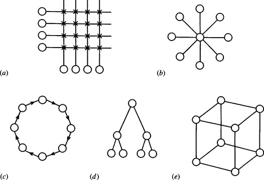
Figure 28.2 Possible arrangements for linking processing elements: (a) crossbar; (b) star; (c) ring; (d) tree; (e) hypercube. All links are bidirectional except where arrows indicate otherwise.
Finally, we should note that factors other than speed enter into the choice of an architecture. For example, many observers have argued that the pyramid type of architecture closely matches the hierarchical data structures most appropriate for scene interpretation.
Much of our discussion has been in the realm of the possible and the ideal (many of the existing systems being expensive experimental ones). It is now necessary to consider more practical issues. How, for example, are we to match the architecture to the data? More particularly, how do we lay down general guidelines for partitioning the tasks and implementing them on practical architectures? In the absence of general guidelines of this type, it is useful to look in detail at a given practical problem to see how to design an optimal hardware system to implement it; this is done in the next section.
28.6 Optimal Implementation of an Image Analysis Algorithm
The particular algorithm considered in this section was examined earlier by Davies and Johnstone (1986, 1989). It involves the inspection of round food products (see also Chapter 22). The purpose of the analysis is to show how to make a systematic selection between available hardware modules (including computers), so that it can be guaranteed that the final hardware configuration is optimal in specific ways and in particular with regard to relevant cost–speed tradeoffs.
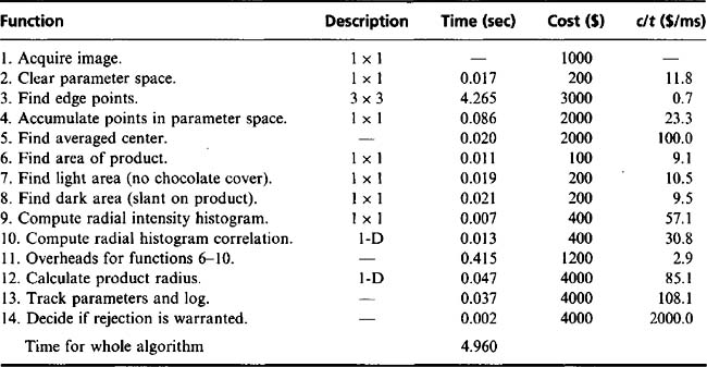
In the particular food product application considered, biscuits are moving at rates of up to 20 per second along a conveyor. Since the conveyor is moving continuously, it is natural to use a line-scan camera to obtain images of the products. Before they can be scrutinized for defects and their sizes measured, they have to be located accurately within the images. Since the products are approximately circular, it is straightforward to employ the Hough transform technique for the purpose (see Chapter 10). It is also appropriate to use the radial intensity histogram approach to help with the task of product scrutiny (Chapter 22). In addition, simple thresholding can be used to measure the amount of chocolate cover and certain other product features. The main procedures in the algorithm are summarized in Table 28.1. Note that the Hough transform approach requires the rapid and accurate location of edge pixels, which is achieved using the Sobel operator and thresholding the resulting edge enhanced image. Edge detection is in fact the only 3 × 3 neighborhood operation in the algorithm and hence it is relatively time-consuming; rather less processing is required by the 1 × 1 neighborhood operations (Table 28.1). Then come various 1-D processes such as analysis of radial histograms. The fastest operations are those such as logging variables, which are neither 1-D nor 2-D processes.
28.6.1 Hardware Specification and Design
On finalization of the algorithm strategy, the overall execution time was found to be about 5 seconds per product (Davies and Johnstone, 1986).3 With product flow rates on the order of 20 per second, and software optimization subject to severely diminishing returns, a further gain in speed by a factor of around 100 could be obtained only by using special electronic hardware. In this application, a compromise was sought with a single CPU linked to a set of suitable hardware accelerators. In this case, the latter would have had to be designed specially for the purpose, and indeed some were produced in this way. However, in the following discussion it is immaterial whether the hardware accelerators are made specially or purchased: the object of the discussion is to present rigorous means for deciding which software functions should be replaced by hardware modules.
As a prerequisite to the selection procedure, Table 28.1 lists execution times and hardware implementation costs of all the algorithm functions. The figures are somewhat notional since it is difficult to divide the algorithm rigorously into completely independent sections. However, they are sufficiently accurate to form the basis for useful decisions on the cost-effectiveness of hardware. Because the aim is to examine the principles underlying cost–speed tradeoffs, the figures presented in Table 28.1 are taken as providing a concrete example of the sort of situation that can arise in practice.
28.6.2 Basic Ideas on Optimal Hardware Implementation
The basic strategy that was adopted for deciding on a hardware implementation of the algorithm is as follows:
1. Prioritize the algorithm functions so that it is clear in which order they should be implemented.
2. Find some criterion for deciding when it is not worth proceeding to implement further functions in hardware.
From an intuitive point of view, function prioritization seems to be a simple process. Basically, functions should be placed in order of cost-effectiveness; that is, those saving the most execution time per unit cost (when implemented in hardware) should be placed first, and those giving smaller savings should be placed later. Thus, we arrive at the c/t (cost/time) criterion function. Then with limited expenditure we achieve the maximum savings in execution time, that is, the maximum speed of operation.
To decide at what stage it is not worth implementing further functions in hardware is arguably more difficult. Excluding here the practical possibility of strict cost or time limits, the ideal solution results in the optimal balance between total cost and total time. Since these parameters are not expressible in the same units, it is necessary to select a criterion function such as C × T (cost × time) which, when minimized, allows a suitable balance to be arrived at automatically.
The procedure outlined here is simple and does not take account of hardware which is common to several modules. This “overhead” hardware must be implemented for the first such module and is then available at zero cost for subsequent modules. In many cases a speed advantage results from the use of overhead hardware. In the example system, it is found that significant economies are possible when implementing functions 6 to 10, since common pixel scanning circuitry may be used. In addition, note that any of these functions that are not implemented in hardware engender a time overhead in software. This, and the fact that the time overhead is much greater than the sum of the software times for functions 6 to 10, means that once the initial cost overhead has been paid it is best (at least, in this particular example) to implement all these functions in hardware.
Trying out the design strategy outlined above gives the c/t ratio sequence shown in Table 28.2. A set of overall times and costs resulting from implementing in hardware all functions down to and including the one indicated is now deduced. Examination of the column of C × T products then shows where the tradeoff between hardware and software is optimized. This occurs here when the first 13 functions are implemented in hardware.
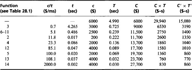
The analysis presented in this section gives only a general indication of the required hardware–software tradeoff. Indeed, minimizing C × T indicates an overall “bargain package,” whereas in practice the system might well have to meet certain cost or speed limits. In this food product application, it was necessary to aim at an overall cost of less than $15,000. By implementing functions 1, 3, and 6 to 11 in hardware, it was found possible to get to within a factor 3.6 of the optimal C × T product. Interestingly, by using an upgraded host processor, it proved possible to get within a much smaller factor (1.8) of the optimal tradeoff, with the same number of functions implemented in hardware (Table 28.2). It is a particular advantage of using this criterion function approach that the choice of which processor to use becomes automatic.
The paper by Davies and Johnstone (1989) goes into some depth concerning the choice of criterion function, showing that more general functions are available and that there is a useful overriding geometrical interpretation—that global concavities are being sought on the chosen curve in f(C), g(T) space. The paper also places the problem of overheads and relevant functional partitions on a more rigorous basis. Finally, a later paper (Davies et al., 1995) emphasizes the value of software solutions, achieved, for example, with the aid of arrays of DSP chips.
28.7 Some Useful Real-time Hardware Options
In the 1980s, real-time inspection systems typically had many circuit boards containing hundreds of dedicated logic chips, though some of the functionality was often implemented in software on the host processor. This period was also a field-day for the Transputer type of microprocessor which had the capability for straightforward coupling of processors to make parallel processing systems. In addition, the “bit-slice” type of microprocessor permitted easy expansion to larger word sizes, though the technology was also capable of use in multipixel parallel processors. Finally, the VLSI type of logic chip was felt by many to present a route forward, particularly for low-level image processing functions.
In spite of all these competing lines, what gradually emerged in the late 1990s as the predominant real-time implementation device was the digital signal processing (DSP) chip. This had evolved earlier in response to the need for fast 1-D signal processors, capable of performing such functions as Fast Fourier Transforms and processing of speech signals. The reason for its success lay in its convenience and programmability (and thus flexibility) and its high speed of operation. By coupling DSP chips together, it was found that 2-D image processing operations could be performed both rapidly and flexibly, thereby to a large extent eliminating the need for dedicated random logic boards, and at the same time ousting Transputers and bit-slices.
Over the same period, however, single-chip Field-Programmable Logic Arrays (FPGAs) were becoming more popular and considerably more powerful, while, in the 2000s, microprocessors are even being embedded on the same chip. At this stage, the concept is altogether more serious, and in the 2000s one has to think very carefully to obtain the best balance between DSP and FPGA chips for implementing practical vision systems.
Another contender in this race is the ordinary PC. While in the 1990s the PC had not normally been regarded as a suitable implementation vehicle for real-time vision, the possibility of implementing some of the slower real-time functions using a PC gradually arose though the relentless progression of Moore’s Law. At the same time, other work on special software designs (see Chapter 23) showed how this line of development could be extended to faster running applications. At the time of writing, it can be envisaged that a single unaided PC—with a reliable embedded operating system—will, by the end of the decade, be sufficient to run a large proportion of all machine vision applications. Indeed, this is anticipated by many sectors of industry. Although it is always risky to make predictions, we can at least anticipate that in the next 10 years the whole emphasis of real-time vision will move away from speed being the dominating influence. At that stage effectiveness, accuracy, robustness, and reliability (what one might call “fitness for purpose”) will be all that matters. For the first time we will be free to design ideal vision systems. The main word of caution is that this ideal will not necessarily apply for all possible applications—one can imagine exceptions, for example, where ultra–high speed aircraft have to be controlled or where huge image databases have to be searched rapidly.
Overall, we can see a progression amid all the hardware developments outlined here. This is a move from random logic design to use of software-based processing elements, and further, one where the software runs not on special devices with limited capability but on conventional computers for which (1) very long instruction words are not needed, (2) machine code or assembly language programming is not necessary to get the most out of the system (so standard languages can be used), and (3) overt parallel processing (beyond that available in the central processing chip of a standard PC) is no longer crucial.4 The advantages in terms of flexibility are dramatic compared with the early days of machine vision.
The trends described here are underlined by the publications discussed in Section 28.13.2 and are summarized in Table 28.3.
Table 28.3 Hardware devices for the implementation of vision algorithms
| Device | Function | Summary of properties |
|---|---|---|
| PC | Personal computer or more powerful workstation: complete computer with RAM, hard disc, and other peripheral devices. Would need an embedded (restricted) operating system in a real-time application. | |
| MP | Microprocessor: single chip device containing CPU+cache RAM. The core element of a PC. | |
| DSP | Digital signal processor: long instruction word MP chip designed specifically for signal processing—high processing speed on a restricted architecture. | |
| FPGA | Field programmable gate array: random logic gate array with programmable linkages; may even be dynamically reprogrammable within the application. The latest devices have flip-flops and higher level functions already made up on chip, ready for linking in; some such devices even have one or more MPs on board. | |
| LUT | Lookup table: RAM or ROM. Useful for fast lookup of crucial functions. Normally slave to a MP or DSP. | |
| ASIC | Application specific integrated circuit: contains devices such as Fourier Transforms, or a variety of specific SP or Vision functions. Normally slave to a MP or DSP. | |
| Vision chip | Vision chips are ASICs that are devised specifically for vision: they may contain several important vision functions, such as edge detectors, thinning algorithms, and connected components analyzers. Normally slave to an MP or DSP. | |
| VLSI | Custom VLSI chip: this commonly has many components from gate level upwards frozen into a fixed circuit with a particular functional application in mind. (Note, however, that the generic name includes MPs, DSPs, though we shall ignore this possibility here.) |
The only high-cost item is the VLSI chip; the cost of producing the masks is only justifiable for high-volume products, such as those used in digital TV. In general, high cost means more than $15,000, medium cost means around $3000, and low cost means less than $150.
If there is a single winner in this table from the point of view of real-time applications, it is the FPGA, supposing only that it contains sufficient on-board raw computing power to make optimum use of its available random logic. Its dynamic reprogrammability is potentially extremely powerful, but it needs to be known how to make best use of it. It has been usual to slave FPGAs to DSPs or MPs,1 but the picture changes radically for FPGAs containing on-chip MPs.
28.8 Systems Design Considerations
Having focused on the problems of real-time hardware design, we now need to get a clearer idea of the overall systems design process. One of the most important limitations on the rate at which machine vision systems can be produced is the lack of flexibility of existing design strategies. This applies especially for inspection systems. To some extent, this problem stems from lack of understanding of the basic principles of vision upon which inspection systems might optimally be based. In addition, there is the problem of lack of knowledge of what goes into the design process. It is difficult enough designing a complete inspection system, including all the effort that goes into producing a cost-effective real-time hardware implementation, without having to worry at the same time whether the schema used is generic or adaptable to other products. Yet this is a crucial factor that deserves a lot of attention.
A major factor standing in the way of progress in this area is the lack of complete case studies of inspection systems. This problem arises partly from lack of detailed knowledge of existing commercial systems and partly from lack of space in journal or conference papers. In the case of conference papers what suffers is published know-how—particularly on creativity aspects. (Journals see their role as promoting scientific methodology and results rather than subjective design notions.) Nevertheless, subjective notions are part of the whole design process, and if the situation is to develop as it should, the mental background should be aired as part of the overall design procedure. We summarize the situation in the following section.
28.9 Design of Inspection Systems—The Status Quo
As practiced hitherto, the design of an inspection system has a number of stages, much as in the list presented in Table 28.4. Although this list is incomplete (e.g., it includes no mention of lighting systems), it is a useful start, and it does reveal something about the creativity aspects—by admitting that reassessments of the efficacy of algorithms may be needed. There are necessarily one or two feedback loops, through which the efficacy can be improved systematically, again and again, until operation is adequate, or indeed until the process is abandoned.5 The underlying process appears to be:
Table 28.4 Stages in the design of a typical inspection system
| 1. Hearing about the problem |
| 2. Analyzing the situation |
| 3. Looking at the data |
| 4. Testing obvious algorithms |
| 5. Realizing limitations |
| 6. Developing algorithms further |
| 7. Finding things are difficult and to some extent impossible |
| 8. Doing theory to find the source of any limitations |
| 9. Doing further tests |
| 10. Getting an improved approach |
| 11. Reassessing the specification |
| 12. Deciding whether to go ahead |
| 13. Completing a software system |
| 14. Assessing the speed limitations |
| 15. Starting again if necessary |
| 16. Speeding up the software |
| 17. Reaching a reasonable situation |
| 18. Putting through 1000 images |
| 19. Designing a hardware implementation |
| 20. Revamping the software if necessary |
| 21. Putting through another 100,000 images |
| 22. Assessing difficulties regarding rare events |
| 23. Assessing timing problems |
| 24. Validating the final system |
The “if no further ideas” clause can be fulfilled if no way is found of making the system fast enough or low enough in cost, or of high enough specification. This would account for most contingencies that could arise.
The problem with the above process is that it represents ad hoc rather than scientific development, and there is no guarantee that the solution that is reached is optimal. Indeed, specification of the problem is not insisted upon (except to the level of adequacy), and if specification and aims are absent, it is impossible to judge whether or not the success that is obtained is optimal. In an engineering environment we ought to insist on problem specification first, solution second. However, things are more complex than this discussion would imply—as will be seen from Table 28.5.
Table 28.5 Complexities of the design process
| • It is not always evident that there is a solution, or at least a cost-effective one. |
| • Specifications cannot always be made in a nonfuzzy manner. |
| • There is often no rigorous scientific design procedure to get from specification to solution. (There is certainly no guaranteed way of achieving this optimally.) |
| • The optimization parameters are not obvious; nor are their relative priorities clear. |
| • It can be quite difficult to discern whether one solution is better than another. |
| • Some inspection environments make it difficult to tell whether or not a solution is valid. |
The last case in Table 28.5 illustrates some types of faults6 that are particularly rare, so that only one may arise in many millions of cases, or, equivalently, every few weeks or months. Thus there is little statistical basis for making judgments of the risk of failure, and there is no proper means of training the system so that it can learn to discriminate these faults. For these reasons, making a rigorous specification and systematically trying to meet it are extremely difficult, though it is still worth trying to do so.
Let us return to the first of the complexities listed in Table 28.5. Although in principle it is difficult to know whether there is a solution to a problem, nevertheless it is frequently possible to examine the computer image data that arise in the application and to see whether the eye can detect the faults or the foreign objects. If it can, this represents a significant step forward, for it means that it should be possible to devise a computer algorithm to do the same thing. What will then be in question will be whether we are creative enough to design such an algorithm and to ensure that it is sufficiently rapid and cost-effective to be useful.
A key factor at this point is making an appropriate choice of design strategy: with structured types of image data. For example, we can ask the following:
Which of these alternatives could, with the particular dataset, lead to algorithms of appropriate speed and robustness? On the other hand, for data that are fuzzy or where objects are ill-defined, would artificial neural networks be more useful than conventional programming? Overall, the types of data, and the types of noise and background clutter that accompany it, are key to the final choice of algorithm.
28.10 System Optimization
To proceed further, we need to examine the optimization parameters that are relevant. There are arguably rather few of these:
These one-word parameters are as yet rather imprecise. For example, reliability can mean a multitude of things, including freedom from mechanical failures such as might arise with the camera being shaken loose, or the illumination failing; or where timing problems occur when additional image clutter results in excessive analysis time, so that the computer can no longer keep up with the real-time flow of product. Several of the parameters have been shown to depend upon each other—for example sensitivity and accuracy, cost, and speed: more will be said about this matter in Chapter 29. Thus, we are working in a multidimensional space with various constraining curves and surfaces. In the worst case, all the parameters will be interlinked, corresponding to a single constraining surface, so that adjusting one parameter forces adjustment of at least one other. It is also possible that the constraining surface will impose hard limits on the values of some parameters.
Each algorithm will have its own constraining surface, which will in general be separate from that of others. Placing all such surfaces together will create some sort of envelope surface, corresponding to the limits of what is possible with currently available algorithms (Fig. 28.3). There will also be an envelope surface, corresponding to what is possible with all possible algorithms, that is, including those that have not yet been developed. Thus, there are limits imposed by creativity and ingenuity, and of course it is not known at what stage, if ever, such limits might be overcome.
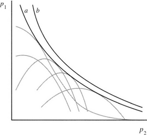
Figure 28.3 Optimization curves for a two-parameter system. The gray curves result from individual algorithms. (a) is the envelope of the curves for all known algorithms. (b) is the limiting curve for all possible algorithms.
Returning to the constraining surface, we can see that it provides an element of choice in the situation. Do we prefer a sensitive algorithm or a robust one, a reliable algorithm or a fast one? And so on. However, algorithms are rarely accurately describable as robust or nonrobust, reliable or nonreliable; the multiparameter space concept with its envelope constraining surfaces clearly allows for variations in such parameters. But at the present stage of development of the subject, the problem we have is that these constraining surfaces are, with few exceptions, unknown, and the algorithms that could provide access to their ideal forms are also largely unknown. Even the algorithms that are available are of largely unmapped capabilities. Also, means are not generally known for selecting optimal working points. (An interesting exception is that elucidated by Davies and Johnstone (1989) relating to optimization of cost/speed tradeoffs for image processing hardware.) Thus, there is a long way to go before the algorithm design and selection process can be made fully scientific.
28.11 The Value of Case Studies
In the absence of scientific know-how, we may be best advised to go for a case-law situation, in which we carefully define the regions where given algorithms are thought to be optimal. Thus, one case study will make one claim, and another case study will make another claim. If two algorithms overlap in their regions of applicability, then it may be possible to prove that the first is, in that region, superior to the second, so that the second can be dispensed with. However, methods usually have different regions of applicability so that the one is not a subset of the other, and then both methods have to be retained independently.
It more often happens that the regions of applicability are not so precisely known or specified. At this point, let us consider inherently simple situations where objects are to be located against blank backgrounds. The only interfering factors are noise and other objects of the same type. Even here, we must appreciate that the noise may be partly Gaussian, partly impulse, partly white, partly periodic, it may also vary from one part of the image to another; and it may vary in a complex way with the gray-scale quantization. In addition, the intensity range may be wide or narrow, compressed at one end or the other, subject to exponential (as in X-ray images) or other laws, and subject to shadows or glints as well as the type of object in question. Then the objects themselves may be separate, touching, overlapping, subject to differing variabilities—in size, shape, orientation, distortion, and so on. There may be a great many of these objects or just a few; they may be small, scattered randomly, arranged in piles, appear to form a texture, and may be unsegmentable in the images. Thus, even in this one “simple” example, the potential variability is so great that it may be extremely difficult to write down all the variables and parameters of the input data so that we know exactly when a given algorithm or suite of algorithms will give an optimal solution.
Small wonder, then, that workers often seem to be reinventing the wheel. They may have worked diligently trying to get a previously available algorithm to work with their particular dataset, only to discover some major deficiency. And then, further work will have shown an appropriate route to take, with yet another algorithm which is a priori apparently unnecessary. So much for the adaptability that was advocated earlier in this chapter—the matter is far less trivial than might have been imagined.
Exploring the situation further, we can find even low-level algorithms difficult to design and specify rigorously. The noise and intensity range problems referred to earlier still seem not to have been solved satisfactorily. We would be hard pressed to describe these problems quantitatively, and if we cannot do even this, how can we be confident of anything? In particular, if we knew that impulse and Gaussian noise were at specifiably low levels, we could confidently apply thresholding algorithms and then proceed to perform shape analysis by skeletonization techniques. Unfortunately, this degree of confidence may rarely be justifiable. Thus, the odd small hole may appear in a binary shape, thereby significantly altering its skeleton. This will then radically alter the range of solutions that may realistically be adopted for image analysis.7
How, then, are we to develop the subject properly and make it more scientific? We must adopt the strategy of gathering as much precise information as possible, mostly with regard to individual cases we will be working on. For each case study we should write out working profiles in as much detail as possible and publish a substantial proportion of the available data. It can’t be emphasized enough that a lot of information should be provided defining the type of image data on which any algorithm has worked. By doing all this, we will at least be mapping out the constraint regions for each algorithm in the relevant parameter space in relation to the specific image data. Later, it should be possible to analyze all such mappings carefully. Important lessons will then be learned about when individual algorithms and techniques should properly be used. These ideas make some responses to the important statements in the earlier literature of the subject, which seem, unfortunately, to have yet had relatively little effect on most workers in the field (Jain and Binford, 1991; Haralick, 1992; Pavlidis, 1992). This lack of effect—especially with regard to Haralick’s work—is probably due to the workers’ awareness of the richness of the data and the algorithmic structures needed to cope rigorously with it, and in the face of such complexity, no one has quite seen how to proceed.
28.12 Concluding Remarks
This chapter has studied the means available for implementing image analysis and inspection algorithms in real time. Fast sequential and various parallel processing architectures have been considered, as well as other approaches involving use of DSP and FPGA chips, or even PCs with embedded operating systems. In addition, means of selecting between the various realizable schemes have been studied, these means being based on criterion function optimizations.
The field is characterized on the one hand by elegant parallel architectures that would cost an excessive amount in most inspection applications and on the other by hardware solutions that are optimized to the application and yet are bound to lack generality. It is easy to gain too rosy a view of the elegant parallel architectures that are available. Their power and generality could easily make them an overkill in dedicated applications, while reductions in generality could mean that their PEs spend much of their time waiting for data or performing null operations. Overall, the subject of image analysis is quite variegated and it is difficult to find a set of “typical” algorithms for which an “average” architecture can be designed whose PEs will always be kept usefully busy. Thus, the subject of mapping algorithms to architectures—or, better, of matching algorithms and architectures—that is, designing them together as a system—is a truly complex one for which obvious solutions turn out to be less efficient in reality than when initially envisioned. Perhaps the main problem lies in envisaging the nature of image analysis, which in the author’s experience turns out to be a far more abstract process than image processing (i.e., image-to-image transformation) ideas would indicate (see especially Chapter 6).
Interestingly, the problems of envisaging the nature of image analysis and of matching hardware to algorithms are gradually being bypassed by the relentless advance in the speed and power of everyday computers. There will be less need for special dedicated hardware for real-time implementation, especially if suitable algorithms such as those outlined in Section 23.4 can be developed. All this represents a very welcome factor for those developing vision systems for industry.
One topic that has been omitted for reasons of space is that of carrying out sufficiently rigorous timing analysis of image analysis and related tasks so that the overall process is guaranteed to run in real time. In this context, a particular problem is that unusual image data conditions could arise that might engender additional processing, thereby setting the system behind schedule. This situation could arise because of excessive noise, because more than the usual number of products appear on a conveyor, because the heuristics in a search tree prove inadequate in some situation, or for a variety of other reasons. One way of eliminating this type of problem is to include a watchdog timer, so that the process is curtailed at a particular stage (with the product under inspection being rejected or other suitable action being taken). However, this type of solution is crude, and sophisticated timing analysis methods now exist, based on Quirk analysis. Môtus and Rodd are protagonists of this type of rigorous approach. The reader is referred to Thomas et al. (1995) for further details and to Môtus and Rodd (1994) for an in-depth study.
Finally, the last few sections have highlighted certain weaknesses in the system design process and indicated how the subject can be developed further for the benefit of industry. Perusal of the earlier chapters will quickly show that we can now achieve quite a lot even though our global design base is limited. The key to our ability to solve the problems, and to know that they are solvable, lies in the ability of the human visual system to carry out relevant visual tasks. Note, however, that there is sound reason for replacing the human eye for these visual tasks—so that (for example) 100% tireless inspection can be carried out and so that it can be achieved consistently and reliably to known standards.
The greatest proportion of the real-time vision system design process used to be devoted to the development of dedicated hardware accelerators. This chapter has emphasized that this problem is gradually receding, and that it is already possible to design reconfigurable FPGA systems that in many cases bypass the need for any special parallel processor systems.
28.13 Bibliographical and Historical Notes8
28.13.1 General Background
The problem of implementing vision in real time presents exceptional difficulties because in many cases megabytes of data have to be handled in times of the order of hundredths of a second, and often repeated scrutiny of the data is necessary. Probably it is no exaggeration to say that hundreds of architectures have been considered for this purpose, all having some degree of parallelism. Of these, many have highly structured forms of parallelism, such as SIMD machines. The idea of an SIMD machine for image parallel operations goes back to Unger (1958) and strongly influenced later work both in the United Kingdom and the United States. For an overview of early SIMD machines, see Fountain (1987).
The SIMD concept was generalized by Flynn (1972) in his well-known classification of computing machines (Section 28.5), and several attempts have been made to devise a more descriptive and useful classification (see Hockney and Jesshope, 1981), although so far none has really caught on (however, see Skillicorn, 1988, for an interesting attempt). Arguably, this is because it is all too easy for structures to become too lacking in generality to be useful for a wide range of algorithmic tasks. There has been a great proliferation of interconnection networks (see Feng, 1981). Reeves (1984) reviewed a number of such schemes that might be useful for image processing. An important problem is that of performing an optimal mapping between algorithms and architectures, but for this to be possible a classification of parallel algorithms is needed to complement that of architectures. Kung (1980) made a start with this task. This work was extended by Cantoni and Levialdi (1983) and Chiang and Fu (1983).
For one period in the 1980s it became an important challenge to design VLSI chips for image processing and analysis. Offen (1985) summarized many of the possibilities, and this work was followed by Fountain’s (1987) volume. The problems targeted in that era were defining the most useful image processing functions to encapsulate in VLSI and to understand how best to partition the algorithms, taking account of chip limitations. At a more down-to-earth level, many image processing and analysis systems did not employ sophisticated parallel architectures but “merely” very fast serial processing techniques with hard-wired functions—often capable of processing at video rates (i.e., giving results within one TV frame time).
During the late 1980s, the Transputer provided the system implementer with a powerful processor with good communication facilities (four bidirectional links each with the capability for independent communication at rates of 10 Mbits per second and operation independent of the CPU), enabling him or her to build SIMD and MIMD machines on a do-it-yourself basis. The T414 device had a 32-bit processor operating at 10 MIPS with a 5 MHz clock and 2 kB of internal memory, while the T800 device had 4 kB of internal memory and a floating-point processor (Inmos, 1987), yet it cost only around $300. These devices were incorporated in a number of commercially available board-level products plus a few complete rather powerful systems; vision researchers developed parallel algorithms for them, using mainly the Occam parallel processing language (Inmos 1988; Pountain and May, 1987).
Other solutions included the use of bit-slice types of device (Edmonds and Davies, 1991), and DSP chips (Davies et al., 1995), while special-purpose multiprocessor designs were described for implementing multiresolution and other Hough transforms (Atiquzzaman, 1994).
28.13.2 Recent Highly Relevant Work
As indicated in Section 28.7, VLSI solutions to the production of rapid hardware for real-time applications have gradually given way to the much more flexible software solutions permitted by DSP chips and to the highly flexible FPGA type of system that permits random logic to be implemented with relative ease. FPGAs offer the possibility of dynamic reconfigurability, which may ultimately be very useful for space probes and the like, though it may prove to be an unnecessary design burden for most vision applications. Better instead to keep on upgrading a design and extending the number of FPGA chips until the required degree of sophistication and speed has been achieved.9 In this respect, it is interesting to note that the current trend is toward hybrid CPU/FPGA chips (Andrews et al., 2004), which will have optimal combinations of software and random logic available awaiting software and hardware programming (see also Batlle et al., 2002).
Be this as it may, in the early 2000s considerable attention was still focused on VLSI solutions to vision applications (Tzionas, 2000; Mémin and Risset, 2001; Wiehler et al., 2001; Urriza et al., 2001), and it is clear that there are bound to be high-volume applications (such as digital television) where this will remain the best approach. Similarly, a lot of attention is still focused on SIMD and on linear array processor schemes, as there will always be facilities that offer ultra-high-speed solutions of this type. In any case, small-scale implementations are likely to be cheap and usable for those (mainly low-level vision) applications that match this type of architecture. Examples appear in the papers by Hufnagl and Uhl (2000), Ouerhani and Hügli (2003), and Rabah, et al. (2003).
Moving on to FPGA solutions, we find these embodying several types of parallelism and applied to underwater vision applications and robotics (Batlle, et al., 2002), subpixel edge detection for inspection (Hussmann and Ho, 2003), and general low-level vision applications, including those implementable as morphological operators (Draper et al., 2003).
DSP solutions, some of which also involve FPGAs, include those by Meribout et al. (2002) and Aziz et al. (2003). It is useful to make comparisons with the Datacube MaxPCI (containing a pipeline of convolvers, histogrammers, and other devices) and other commercially available boards and systems—see Broggi et al. (2000a, b), Yang et al. (2002), and Marino et al. (2001). The Marino et al. paper is exceptional in using a clever architecture incorporating extensive use of lookup tables to perform high-speed matching functions that lead to road following. The matching functions involve location of interest points, followed by high-speed search for matching them between corresponding blocks of adjacent frames. This should be regarded as an application of quite simple low-level operations that enable high-level operations to take place quickly. An interesting feature is the use of a residue number system to (effectively) factorize large lookup tables into several much smaller and more manageable lookup tables.
1 Sometime in the future this view will need to be reconsidered; see Section 28.7.
2 In this context, it is conventional to use the term bandwidth to mean the maximum rate realizable via the stated mechanism.
3 Although the particular example is dated, the principles involved are still relevant and are worth following here.
4 Nevertheless, some functions such as image acquisition and control of mechanical devices will have to be carried out in parallel, to prevent data bottlenecks and other holdups.
1 In fact, the FPGA and the DSP complement each other exceptionally well, and it has been common practice to use them in tandem.
5 It is in the nature of things that you can’t be totally sure whether a venture will be a success without trying it. Furthermore, in the hard world of industrial survival, part of adequacy means producing a working system and part means making a profit out of it. This section must be read in this light.
6 An important class of rare faults is that of foreign objects, including the hard and sometimes soft contaminants targeted by X-ray inspection systems.
7 Intrinsically, a skeleton gives a good indication of the shape of an object. Furthermore, if one noise point produces an additional loop in a skeleton, this could possibly be coped with by subsequent analysis procedures. However, significant numbers of noise points will add so much additional complexity to a skeleton that a combinatorial explosion of possible solutions will occur, with the result that the skeleton will no longer be a useful representation of the underlying shape of the object.
8 Because of the rapid ageing process that is particularly evident for computer and hardware development, it has been found necessary to divide this section into two parts “General Background” (including early work) and “Recent Highly Relevant Work.”
9 However, see Kessal et al. (2003) for a highly interesting investigation of the possibilities—in particular showing that dynamic reconfigurability of a real-time vision system can already be achieved in milliseconds.