Search in book...
Toggle Font Controls
Create new playlist

Name your new playlist

Playlist description (optional)
Sign In

Email address

Password

Forgot Password?

or

Continue with Facebook

Continue with Google
Sign Up

Full Name

Email address

Confirm Email Address

Password

or

Continue with Facebook

Continue with Google

Spherical Waves and Applications

5
Spherical Waves and Applications

So far, we have discussed plane waves and cylindrical waves. In both of these cases, we could develop with relative ease the solutions based on TM^z and TE^z modes. We illustrated these solutions by solving some waveguides and cavity problems. The superscript z is added here to indicate that the transverse plane is perpendicular to the z-coordinates. The structures under consideration had a uniform cross section for all values of z. In spherical coordinates, we do not have any such transverse planes, and thus spherical wave problems are mathematically more involved. It is still possible to have mode classification as TM^r and TE^r.

The solution in spherical coordinates involves special functions: spherical Bessel functions and associated Legendre functions. Spherical Bessel functions are related to half-integral Bessel functions.

5.1Half-Integral Bessel Functions

In connection with the solution for a scalar Helmholtz equation in spherical coordinates, we come across the differential equation

(5.1)

u \frac{d}{d u} (u \frac{d f}{d u}) + [u^{2} - {(n + \frac{1}{2})}^{2}] f = 0,

$u \frac{d}{d u} (u \frac{d f}{d u}) + [u^{2} - {(n + \frac{1}{2})}^{2}] f = 0,$

which, when expanded, gives

(5.2)

\frac{d^{2} f}{d u^{2}} + \frac{1}{u} \frac{d f}{d u} + [1 - \frac{{(n + 1 / 2)}^{2}}{u^{2}}] f = 0.

$\frac{d^{2} f}{d u^{2}} + \frac{1}{u} \frac{d f}{d u} + [1 - \frac{{(n + 1 / 2)}^{2}}{u^{2}}] f = 0.$

By comparing with Equation 2.120, we immediately realize that f can be written as a linear combination of half-integral Bessel functions:

(5.3)

f = \{\begin{array}{c} J_{n + 1 / 2} (u) \\ Y_{n + 1 / 2} (u) \\ H_{n + 1 / 2}^{(1)} (u) \\ H_{n + 1 / 2}^{(2)} (u) \\ I_{n + 1 / 2} (u) \\ K_{n + 1 / 2} (u) \end{array}\} .

$f = \{\begin{array}{c} J_{n + 1 / 2} (u) \\ Y_{n + 1 / 2} (u) \\ H_{n + 1 / 2}^{(1)} (u) \\ H_{n + 1 / 2}^{(2)} (u) \\ I_{n + 1 / 2} (u) \\ K_{n + 1 / 2} (u) \end{array}\} .$

Half-integral Bessel functions can be shown to reduce to simpler forms:

(5.4)

J_{n + 1 / 2} (x) = \sqrt{\frac{2}{π}} x^{n + 1 / 2} {(- \frac{1}{x})}^{n} \frac{d^{n}}{d x^{n}} (\frac{sin x}{x}),

$J_{n + 1 / 2} (x) = \sqrt{\frac{2}{π}} x^{n + 1 / 2} {(- \frac{1}{x})}^{n} \frac{d^{n}}{d x^{n}} (\frac{sin x}{x}),$

(5.5)

Y_{n + 1 / 2} (x) = {(- 1)}^{n + 1} \sqrt{\frac{2}{π}} x^{n + 1 / 2} {(\frac{1}{x})}^{n} \frac{d^{n}}{d x^{n}} (\frac{cos x}{x}) .

$Y_{n + 1 / 2} (x) = {(- 1)}^{n + 1} \sqrt{\frac{2}{π}} x^{n + 1 / 2} {(\frac{1}{x})}^{n} \frac{d^{n}}{d x^{n}} (\frac{cos x}{x}) .$

In particular, we can show from Equation 5.4 that

(5.6)

J_{1 / 2} (x) = \sqrt{\frac{2}{π x}} sin x,

$J_{1 / 2} (x) = \sqrt{\frac{2}{π x}} sin x,$

(5.7)

J_{3 / 2} (x) = \sqrt{\frac{2}{π x}} ((\frac{sin x}{x}) - cos x) .

$J_{3 / 2} (x) = \sqrt{\frac{2}{π x}} ((\frac{sin x}{x}) - cos x) .$

From Equations 5.6 and 5.7, we can obtain the zeros of half-integral Bessel functions and their derivatives. These are listed in Tables 5.1 and 5.2.

TABLE 5.1
Zeros of Half-Integral Bessel Functions χ_n+1/2,I

J_1/2	J_3/2	J_5/2
3.1416	4.4934	5.7635
6.2832	7.7253	9.0950

TABLE 5.2
Zeros of Derivatives of Half-Integral Bessel Functions $χ_{n + 1 / 2, I}^{'}$ $χ_{n + 1 / 2, I}^{'}$

$J_{1 / 2}^{'}$ $J_{1 / 2}^{'}$	$J_{3 / 2}^{'}$ $J_{3 / 2}^{'}$	$J_{5 / 2}^{'}$ $J_{5 / 2}^{'}$
1.1656	2.4605	3.6328
4.6042	6.0293	7.3670

5.2Solutions of Scalar Helmholtz Equation

The scalar Helmholtz equations

(5.8)

\nabla^{2} F + k^{2} F = 0

$\nabla^{2} F + k^{2} F = 0$

and

\frac{1}{r^{2}} \frac{\partial}{\partial r} (r^{2} \frac{\partial F}{\partial r}) + \frac{1}{r^{2} sin θ} \frac{\partial}{\partial θ} (sin θ \frac{\partial F}{\partial θ}) + \frac{1}{r^{2} {sin}^{2} θ} \frac{\partial^{2} F}{\partial ϕ^{2}} + k^{2} F = 0

$\frac{1}{r^{2}} \frac{\partial}{\partial r} (r^{2} \frac{\partial F}{\partial r}) + \frac{1}{r^{2} sin θ} \frac{\partial}{\partial θ} (sin θ \frac{\partial F}{\partial θ}) + \frac{1}{r^{2} {sin}^{2} θ} \frac{\partial^{2} F}{\partial ϕ^{2}} + k^{2} F = 0$

can be solved in spherical coordinates by the usual technique of separation of variables. Let

(5.9)

F = (r, θ, ϕ) = f_{1} (r) f_{2} (θ) f_{3} (ϕ) .

$F = (r, θ, ϕ) = f_{1} (r) f_{2} (θ) f_{3} (ϕ) .$

Substituting Equations 5.9 into 5.8 and manipulating the equation, we obtain the ordinary differential equations for f₁, f₂, and f₃ involving two separation constants m and n:

(5.10)

\frac{d}{d r} (\frac{r^{2} d f_{1}}{d r}) + [k^{2} r^{2} - n (n + 1)] f_{1} = 0,

$\frac{d}{d r} (\frac{r^{2} d f_{1}}{d r}) + [k^{2} r^{2} - n (n + 1)] f_{1} = 0,$

(5.11)

\frac{1}{sin θ} \frac{d}{d θ} (\frac{sin θ d f_{2}}{d θ}) + [n (n + 1) - \frac{m^{2}}{{sin}^{2} θ}] f_{2} = 0,

$\frac{1}{sin θ} \frac{d}{d θ} (\frac{sin θ d f_{2}}{d θ}) + [n (n + 1) - \frac{m^{2}}{{sin}^{2} θ}] f_{2} = 0,$

(5.12)

\frac{d^{2} f_{3}}{d ϕ^{2}} + m^{2} f_{3} = 0.

$\frac{d^{2} f_{3}}{d ϕ^{2}} + m^{2} f_{3} = 0.$

By substituting

(5.13)

r = \frac{u}{k} and f_{1} = \frac{f}{\sqrt{r}} = \sqrt{\frac{k}{u}} f

$r = \frac{u}{k} and f_{1} = \frac{f}{\sqrt{r}} = \sqrt{\frac{k}{u}} f$

in Equation 5.10, we obtain Equation 5.2, with f thus given by a linear combination of half-integral Bessel functions given by Equation 5.3. The solution for f₁ is given by

(5.14)

f_{1} (r) = \frac{f (u)}{\sqrt{r}} = \frac{f (k r)}{\sqrt{r}} .

$f_{1} (r) = \frac{f (u)}{\sqrt{r}} = \frac{f (k r)}{\sqrt{r}} .$

Defining the spherical Bessel function b_n in terms of the half-integral Bessel functions B_n+1/2, we obtain

(5.15)

b_{n} (k r) = \sqrt{\frac{π}{2 k r}} B_{n + 1 / 2} (k r),

$b_{n} (k r) = \sqrt{\frac{π}{2 k r}} B_{n + 1 / 2} (k r),$

where

b_n stands for any of the spherical Bessel functions j_n, y_n, $h_{n}^{(1)}$ $h_{n}^{(1)}$ , and $h_{n}^{(2)}$ $h_{n}^{(2)}$
B_n+1/2 stands for the half–integral Bessel functions, J_{n + 1/2}, Y_n+1/2, $H_{n + 1 / 2}^{(1)}$ $H_{n + 1 / 2}^{(1)}$ , and $H_{n + 1 / 2}^{(2)}$ $H_{n + 1 / 2}^{(2)}$

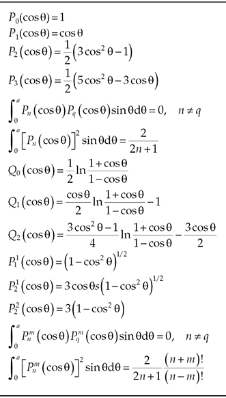
Equation 5.11 is called the associate Legendre equation whose solutions are linear combinations of associate Legendre polynomials of the first kind $(P_{n}^{m})$ $(P_{n}^{m})$ and the second kind $(Q_{n}^{m})$ $(Q_{n}^{m})$ of degree n and order m. These polynomials are given by

(5.16)

P_{n}^{m} (x) = {(x^{2} - 1)}^{m / 2} \frac{d^{m}}{d x^{m}} P_{n} (x),

$P_{n}^{m} (x) = {(x^{2} - 1)}^{m / 2} \frac{d^{m}}{d x^{m}} P_{n} (x),$

(5.17)

P_{n} (x) = \frac{1}{2^{n} n!} \frac{d^{n}}{d x^{n}} {(x^{2} - 1)}^{n},

$P_{n} (x) = \frac{1}{2^{n} n!} \frac{d^{n}}{d x^{n}} {(x^{2} - 1)}^{n},$

(5.18)

Q_{n}^{m} (x) = {(x^{2} - 1)}^{m / 2} \frac{d^{m}}{d x^{m}} Q_{n} (x),

$Q_{n}^{m} (x) = {(x^{2} - 1)}^{m / 2} \frac{d^{m}}{d x^{m}} Q_{n} (x),$

(5.19)

Q_{n} (x) = \frac{1}{2} P_{n} (x) ln \frac{1 + x}{1 - x} - \sum_{l = 1}^{n} \frac{1}{l} P_{l - 1} (x) P_{n - 1} (x) .

$Q_{n} (x) = \frac{1}{2} P_{n} (x) ln \frac{1 + x}{1 - x} - \sum_{l = 1}^{n} \frac{1}{l} P_{l - 1} (x) P_{n - 1} (x) .$

Associated Legendre polynomials of zero order (m = 0) are called Legendre polynomials. In Equation 5.16, Equation 5.17, Equation 5.18 and Equation 5.19, x = cos θ. Note that the order m is an integer between 0 and n. Plots and expressions for a few Legendre polynomials are given in Figure 5.1 and Table 5.3. Note that on the polar axis, that is, θ = 0 or π, Q_n → ∞. So, for the problem that includes a positive or negative polar axis in the field region, the function $P_{n}^{m}$ $P_{n}^{m}$ alone is the suitable solution. The solution for Equation 5.12 is a linear combination of cos mϕ and sin mϕ. Putting together the solutions for f₁, f₂, and f₃, the solution for Equation 5.8 may be written as

(5.20)

F (r, θ, ϕ) = \{\begin{array}{c} j_{n} (k r) \\ y_{n} (k r) \\ h_{n}^{(1)} (k r) \\ h_{n}^{(1)} (k r) \end{array}\} \{\begin{array}{c} P_{n}^{m} (cos θ) \\ Q_{n}^{m} (cos θ) \end{array}\} \{\begin{array}{c} cos m ϕ \\ sin m ϕ \end{array}\} .

$F (r, θ, ϕ) = \{\begin{array}{c} j_{n} (k r) \\ y_{n} (k r) \\ h_{n}^{(1)} (k r) \\ h_{n}^{(1)} (k r) \end{array}\} \{\begin{array}{c} P_{n}^{m} (cos θ) \\ Q_{n}^{m} (cos θ) \end{array}\} \{\begin{array}{c} cos m ϕ \\ sin m ϕ \end{array}\} .$

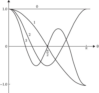
FIGURE 5.1
Polynomials P_n(cos θ). The degree n is indicated on the graph.

5.3Vector Helmholtz Equation

The electric and magnetic fields in a sourceless region satisfy the vector Helmholtz equations

(5.21)

\nabla \times \nabla \times \tilde{E} - k^{2} \tilde{E} = \nabla^{2} \tilde{E} + k^{2} \tilde{E} = 0,

$\nabla \times \nabla \times \tilde{E} - k^{2} \tilde{E} = \nabla^{2} \tilde{E} + k^{2} \tilde{E} = 0,$

(5.22)

\nabla \times \nabla \times \tilde{H} - k^{2} \tilde{H} = \nabla^{2} \tilde{H} + k^{2} \tilde{H} = 0.

$\nabla \times \nabla \times \tilde{H} - k^{2} \tilde{H} = \nabla^{2} \tilde{H} + k^{2} \tilde{H} = 0.$

Each Cartesian component of $\tilde{E}$ $\tilde{E}$ and $\tilde{H}$ $\tilde{H}$ satisfies the scalar Helmholtz equation (5.8), but the spherical components do not satisfy Equation 5.8.

It is convenient once more to think of simple solutions of these equations in terms of TE^r, TM^r, and TEM^r modes in the context of spherical geometry.

5.4TM^r Modes

These modes may be constructed by considering a vector field

(5.23)

\tilde{M} = \nabla \times [\hat{r} r {\tilde{F}}_{e}],

$\tilde{M} = \nabla \times [\hat{r} r {\tilde{F}}_{e}],$

where ${\tilde{F}}_{e}$ ${\tilde{F}}_{e}$ satisfies Equation 5.8. It can be shown that $\tilde{M}$ $\tilde{M}$ satisfies the vector Helmholtz equation. Identifying $\tilde{M}$ $\tilde{M}$ with $\tilde{H}$ $\tilde{H}$ and noting from Equation 5.23 that

(5.24)

H_{r} = 0,

$H_{r} = 0,$

(5.25)

{\tilde{H}}_{θ} = \frac{1}{sin θ} \frac{\partial F_{e}}{\partial ϕ},

${\tilde{H}}_{θ} = \frac{1}{sin θ} \frac{\partial F_{e}}{\partial ϕ},$

(5.26)

{\tilde{H}}_{ϕ} = - \frac{\partial F_{e}}{\partial θ},

${\tilde{H}}_{ϕ} = - \frac{\partial F_{e}}{\partial θ},$

we recognize all the above as the magnetic field components of TM^r modes in terms of the electric Debye potential ${\tilde{F}}_{e}$ ${\tilde{F}}_{e}$ . The corresponding electric field components can be obtained from Maxwell’s equation

(5.27)

\nabla \times \tilde{H} = j ω ε \tilde{E}

$\nabla \times \tilde{H} = j ω ε \tilde{E}$

and are given as

(5.28)

{\tilde{E}}_{r} = - \frac{j}{ω ε} [\frac{\partial^{2}}{\partial r^{2}} r {\tilde{F}}_{e} + k^{2} r {\tilde{F}}_{e}],

${\tilde{E}}_{r} = - \frac{j}{ω ε} [\frac{\partial^{2}}{\partial r^{2}} r {\tilde{F}}_{e} + k^{2} r {\tilde{F}}_{e}],$

(5.29)

{\tilde{E}}_{θ} = - \frac{j}{ω ε} \frac{1}{r} \frac{\partial^{2}}{\partial r \partial θ} r {\tilde{F}}_{e},

${\tilde{E}}_{θ} = - \frac{j}{ω ε} \frac{1}{r} \frac{\partial^{2}}{\partial r \partial θ} r {\tilde{F}}_{e},$

(5.30)

{\tilde{E}}_{ϕ} = - \frac{j}{ω ε} \frac{1}{r sin θ} \frac{\partial^{2}}{\partial r \partial ϕ} r {\tilde{F}}_{e} .

${\tilde{E}}_{ϕ} = - \frac{j}{ω ε} \frac{1}{r sin θ} \frac{\partial^{2}}{\partial r \partial ϕ} r {\tilde{F}}_{e} .$

5.5TE^r Modes

These modes may be constructed by considering the vector function

(5.31)

\tilde{N} = \nabla \times [\hat{r} r {\tilde{F}}_{m}],

$\tilde{N} = \nabla \times [\hat{r} r {\tilde{F}}_{m}],$

where ${\tilde{F}}_{m}$ ${\tilde{F}}_{m}$ satisfies Equation 5.8. It can be shown that $\tilde{N}$ $\tilde{N}$ satisfies the vector Helmholtz equation. Identifying $\tilde{N}$ $\tilde{N}$ with the $\tilde{E}$ $\tilde{E}$ field and noting from Equation 5.31 that

(5.32)

{\tilde{E}}_{r} = 0,

${\tilde{E}}_{r} = 0,$

(5.33)

{\tilde{E}}_{θ} = \frac{1}{sin θ} \frac{\partial F_{m}}{\partial ϕ},

${\tilde{E}}_{θ} = \frac{1}{sin θ} \frac{\partial F_{m}}{\partial ϕ},$

(5.34)

{\tilde{E}}_{ϕ} = - \frac{\partial F_{m}}{\partial θ},

${\tilde{E}}_{ϕ} = - \frac{\partial F_{m}}{\partial θ},$

we recognize the above as the electric field expressions of TE^r modes. The corresponding magnetic field components can be obtained from Maxwell’s equation

(5.35)

\nabla \times \tilde{E} = - j ω μ \tilde{H}

$\nabla \times \tilde{E} = - j ω μ \tilde{H}$

and are given by

(5.36)

{\tilde{H}}_{r} = \frac{j}{ω μ} [\frac{\partial^{2}}{\partial r^{2}} r {\tilde{F}}_{m} + k^{2} r {\tilde{F}}_{m}],

${\tilde{H}}_{r} = \frac{j}{ω μ} [\frac{\partial^{2}}{\partial r^{2}} r {\tilde{F}}_{m} + k^{2} r {\tilde{F}}_{m}],$

(5.37)

{\tilde{H}}_{θ} = \frac{j}{ω μ} \frac{1}{r} \frac{\partial^{2}}{\partial r \partial θ} r {\tilde{F}}_{m},

${\tilde{H}}_{θ} = \frac{j}{ω μ} \frac{1}{r} \frac{\partial^{2}}{\partial r \partial θ} r {\tilde{F}}_{m},$

(5.38)

{\tilde{H}}_{ϕ} = \frac{j}{ω μ} \frac{1}{r sin θ} \frac{\partial^{2}}{\partial r \partial ϕ} r {\tilde{F}}_{m} .

${\tilde{H}}_{ϕ} = \frac{j}{ω μ} \frac{1}{r sin θ} \frac{\partial^{2}}{\partial r \partial ϕ} r {\tilde{F}}_{m} .$

5.6Spherical Cavity

We illustrate the construction of solutions in spherical coordinates by determining the resonant frequencies of a spherical cavity with PEC boundary conditions at r = a (Figure 5.2).

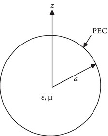
FIGURE 5.2
Spherical cavity with PEC boundary.

For TM modes ${\tilde{F}}_{e}$ ${\tilde{F}}_{e}$ is given by Equation 5.20.

Since θ = 0 or π are part of the field region, we choose $P_{n}^{m}$ $P_{n}^{m}$ for θ variation. Since we need an oscillatory function that is finite at the origin, we choose j_n(kr) for n variation.

The r variation of rF_e is given by

(5.39)

r j_{n} (k r) = r \sqrt{\frac{π}{2 k r}} J_{n + 1 / 2} (k r) = \sqrt{r} \sqrt{\frac{π}{2 k}} J_{n + 1 / 2} (k r) .

$r j_{n} (k r) = r \sqrt{\frac{π}{2 k r}} J_{n + 1 / 2} (k r) = \sqrt{r} \sqrt{\frac{π}{2 k}} J_{n + 1 / 2} (k r) .$

To suit such applications as above, Schelkunoff defined another set of spherical Bessel functions:

(5.40)

{\hat{B}}_{n} (x) = \sqrt{\frac{π x}{2}} B_{n + 1 / 2} (x) .

${\hat{B}}_{n} (x) = \sqrt{\frac{π x}{2}} B_{n + 1 / 2} (x) .$

The roots of ${\hat{J}}_{n} (ζ)$ ${\hat{J}}_{n} (ζ)$ are given in Table 5.4.

TABLE 5.4
Zeros of ${\hat{J}}_{n}$ ${\hat{J}}_{n}$

ζ_np	n = 1	n = 2	n = 3
p = 1	4.493	5.763	6.988
p = 2	7.725	9.095	10.417
p = 3	10.904	12.323	13.698

We may as well now list in Table 5.5 the roots of ${\hat{J}}_{n}^{'} (y) = 0$ ${\hat{J}}_{n}^{'} (y) = 0$ .

TABLE 5.5
Zeros of ${\hat{J}}_{n}^{'}$ ${\hat{J}}_{n}^{'}$

$ζ_{np}^{'}$ $ζ_{np}^{'}$	n = 1	n = 2	n = 3
p = 1	2.744	3.87	4.973
p = 2	6.117	7.443	8.722
p = 3	9.317	10.713	12.064

The PEC boundary conditions are ${\tilde{E}}_{θ} = 0 and {\tilde{E}}_{ϕ} = 0$ ${\tilde{E}}_{θ} = 0 and {\tilde{E}}_{ϕ} = 0$ at r = a, which leads to the boundary condition

(5.41)

{\frac{\partial}{\partial r} (r {\tilde{F}}_{e}) |}_{r = a} = 0, that is, {\hat{J}}_{n}^{'} (k a) = 0,

${\frac{\partial}{\partial r} (r {\tilde{F}}_{e}) |}_{r = a} = 0, that is, {\hat{J}}_{n}^{'} (k a) = 0,$

(5.42)

{(k)}_{n m p}^{T M^{r}} = \frac{ζ_{n p}^{'}}{a},

${(k)}_{n m p}^{T M^{r}} = \frac{ζ_{n p}^{'}}{a},$

(5.43)

{(f_{r})}_{n m p}^{T M^{r}} = \frac{1}{2 π \sqrt{μ ε}} \frac{ζ_{n p}^{'}}{a}, n, p = 1, 2, \dots, \infty .

${(f_{r})}_{n m p}^{T M^{r}} = \frac{1}{2 π \sqrt{μ ε}} \frac{ζ_{n p}^{'}}{a}, n, p = 1, 2, \dots, \infty .$

Note that n cannot be zero since

(5.44)

P_{0}^{0} = 1.

$P_{0}^{0} = 1.$

And from Equations 5.29 and 5.30, ${\tilde{E}}_{θ}$ ${\tilde{E}}_{θ}$ and ${\tilde{E}}_{ϕ}$ ${\tilde{E}}_{ϕ}$ are zero not only on the boundary but also everywhere inside the cavity. Thus, n = 0 gives a trivial solution. The lowest resonant frequency of TM modes is given by

(5.45)

{(f_{r})}_{101}^{T M^{r}} = \frac{1}{2 π \sqrt{μ ε}} \frac{ζ_{11}^{'}}{a} = \frac{2.744}{2 π \sqrt{μ ε} a} .

${(f_{r})}_{101}^{T M^{r}} = \frac{1}{2 π \sqrt{μ ε}} \frac{ζ_{11}^{'}}{a} = \frac{2.744}{2 π \sqrt{μ ε} a} .$

Let us next consider the TE^r modes. The boundary conditions in this case, from Equations 5.33 and 5.34, are

(5.46)

{\frac{\partial F_{m}}{\partial θ} |}_{r = a} = 0,

${\frac{\partial F_{m}}{\partial θ} |}_{r = a} = 0,$

(5.47)

{\frac{\partial F_{m}}{\partial ϕ} |}_{r = a} = 0,

${\frac{\partial F_{m}}{\partial ϕ} |}_{r = a} = 0,$

which translate to

(5.48)

{\hat{J}}_{n} (k a) = 0,

${\hat{J}}_{n} (k a) = 0,$

(5.49)

{(k)}_{n m p}^{T E^{r}} = ζ_{n p},

${(k)}_{n m p}^{T E^{r}} = ζ_{n p},$

(5.50)

{(f_{r})}_{n m p}^{T E^{r}} = \frac{1}{2 π \sqrt{μ ε}} \frac{ζ_{n p}}{a} .

${(f_{r})}_{n m p}^{T E^{r}} = \frac{1}{2 π \sqrt{μ ε}} \frac{ζ_{n p}}{a} .$

The lowest value of the above occurs when n = 1 and p = 1,

(5.51)

{(f_{r})}_{101}^{T E^{r}} = \frac{1}{2 π \sqrt{μ ε}} \frac{4.493}{a} .

${(f_{r})}_{101}^{T E^{r}} = \frac{1}{2 π \sqrt{μ ε}} \frac{4.493}{a} .$

The lowest resonant frequency of all the modes is thus given by Equation 5.45. The modes in a spherical cavity are highly degenerate, that is, for the same resonant frequency we can have many different field distributions.

..................Content has been hidden....................

You can't read the all page of ebook, please click here login for view all page.

Table of Contents for 5. Spherical Waves and Applications

Create new playlist

Sign In

Sign Up

5.1Half-Integral Bessel Functions

5.2Solutions of Scalar Helmholtz Equation

5.3Vector Helmholtz Equation

5.4TMr Modes

5.5TEr Modes

5.6Spherical Cavity

Table of Contents for
5. Spherical Waves and Applications

5.4TM^r Modes

5.5TE^r Modes