
]>
Appendix 6A: On Restricted Fourier Series Expansion
A periodic function expressed by
where T is the period, may be expressed in Fourier series as
In Equation 6A.2,
In trying to solve the Laplace equation in rectangular coordinates with specified boundary conditions, we need Fourier series expansion of an arbitrary function defined over an interval. The boundary conditions may require use of sine terms-only, odd harmonics-only, and so on. The following example [1] illustrates how the function will look in its entire period and what the period is.
Example 6A.1
A function x(t) defined over a finite range 0 < t < t1 is shown in Figure 6A.1.
Sketch the various possible periodic continuations of the function x(t) such that the Fourier series will have
odd harmonics only.
sine terms only.
cosines and odd harmonics only.
sines and odd harmonics only.
The period and continuation of the function in the period are adjusted so as to satisfy the requirements specified.
Solution
For odd harmonics-only, rotational symmetry is required, that is,
(6A.7)The periodic continuation is as shown in Figure 6A.2 with period T = 2t1.
For sine terms-only, odd symmetry is required, that is,
(6A.8)The periodic continuation is as shown in Figure 6A.3 with period T = 2t1 sketched from −t1 to t1.
For cosines and odd harmonics-only, even symmetry and rotational symmetry are required, that is,
(6A.9)The periodic continuation is as shown in Figure 6A.4 with period T = 4t1 sketched from −t1 to 3t1.
For sines and odd harmonics-only, odd symmetry and rotational symmetry are required. That is,
(6A.10)The periodic continuation is as shown in Figure 6A.5 with period T = 4t1 sketched from −t1 to 3t1.

FIGURE 6A.1
A function x(t) defined over the interval 0 < t < t1.

FIGURE 6A.2
x(t) with odd harmonics-only. The dashed curve is x(t − T/2).
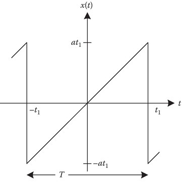
FIGURE 6A.3
x(t) with sine terms-only.

FIGURE 6A.4
x(t) with cosine terms and odd harmonics-only.
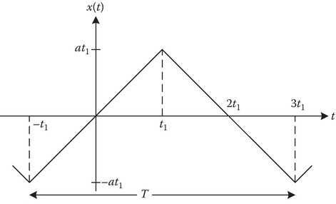
FIGURE 6A.5
x(t) with sine terms and odd harmonics-only.
As an example of the effect of the periodic continuation on the evaluation of the Fourier coefficients, let us take up further the B part for which the period is 2t1. Therefore,
where ω0= 2π/2t1 = π/t1. Since f(t) is odd and sin(nω0t) is odd, the integrand f(t)sin(nω0t) is even for all integral values of n, and therefore,
Reference
- 1.Guillemin, E. A., The Mathematics of Circuit Analysis, Wiley, New York, 1949.