
]>
Appendix 1B: Retarded Potentials and Review of Potentials for the Static Cases
1B.1Electrostatics
The basic equation is
It is known that the curl of the gradient of any scalar is zero, that is,
Therefore, E can be expressed as the gradient of a scalar ψ (electrostatic potential).
where ψ satisfies Poisson’s equation
The solution of Equation 1B.4 at an arbitrary point P is given by
where the volume charge density ρv exists over volume v′ as shown in Figure 1B.1.
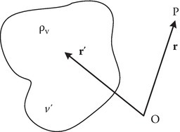
FIGURE 1B.1
Electrostatic geometry.
1B.2Magnetostatics
The basic equation is
It is known that the divergence of the curl of any vector is zero, that is,
Therefore, B can be expressed as the curl of a vector A as
The magnetic vector potential A satisfies the vector Poisson’s equation
In deriving Equation 1B.9, we use Ampere’s law ∇ × H = J and choose ∇ · A = 0. The solution of Equation 1B.9 at an arbitrary point P is given by
and
1B.3Time-Varying Case
We know
and
but
From Equations 1B.13 and 1B.14, we obtain
Therefore, from Equation 1B.2, E + (∂A/∂t) can be expressed as the gradient of a scalar ψ (electric potential)
Now, we shall derive the equations satisfied by A and ψ and we would like to have these equations without the E and H fields in them. We want the equations for the time varying case corresponding to Equations 1B.4 and 1B.9. Let us start with
Using Equations 1B.18, 1B.17, and the relation D = εE, we obtain
Similarly, start from the equation
Since
Equations 1B.20 and 1B.25 are coupled, that is, in each of these equations, both variables ψ and A appear. In the static case, we had uncoupled equations for ψ and A (Equations 1B.4 and 1B.9). A vector is uniquely defined only if its curl and also its divergence are specified everywhere. In the static case, A is made unique by specifying its curl as B, that is, ∇ × A = B, and its divergence as zero, that is, ∇ · A = 0. In the time-varying case, we have specified curl of A as B, but we have not specified its divergence. It is seen from Equation 1B.25 that if we specify (Lorentz condition)
then Equation 1B.25 becomes uncoupled (ψ does not appear in the equation):
Furthermore, if we substitute Equation 1B.26 into Equation 1B.20 to eliminate A, then we obtain
that is,
which is also an uncoupled equation.
Equations 1B.27 and 1B.29 are called wave equations. Although Poisson’s equation governs the static cases, time-varying phenomena are governed by the wave equation.
In free space, 1/ε0μ0 = (3 × 10⁸)2 = c2, where c is the velocity of light. Note that c is large but finite. Equation 1B.29 for free space is
This tends to Equation 1B.4 if 1/c2 → 0, that is, c → ∞. The implication of this statement will be explained later. Consider a charge Q at point A as shown in Figure 1B.2. A comparison between the static and dynamic cases is summarized in Table 1B.1.
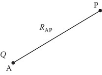
FIGURE 1B.2
Point charge at point A for static and dynamic case comparison.
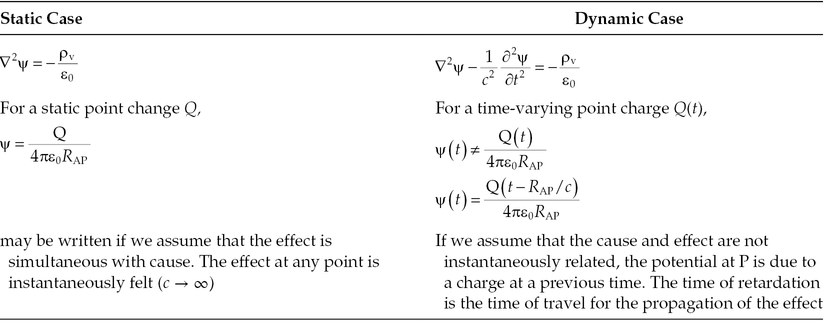
TABLE 1B.1
Comparison of Static and Dynamic Cases for a Point Charge
For a volume charge source of density ρv, the solution is
where
is the charge density at the retarded time.
Example 1B.1
Let a current filament be short (length = ℓ) and carry a current I = I0 cos(ωt) as shown in Figure 1B.3.
Then
For I(t) = I0 cos ωt,
If ℓ ≪ λ,
The phasor Ãz is given by

FIGURE 1B.3
Hertzian dipole.
1B.4One-Dimensional Solution for the Wave Equation
In explaining the retardation effect, we assumed the solution of
is a wave propagating with the velocity c. Let us solve Equation 1B.37 for the one-dimensional case, ψ = ψ (z, t), that is,
Let the Laplace transform of ψ be F and it may be written as
Transforming Equation 1B.37, we obtain
If the initial conditions are zero, then
Then
If and , then by using shifting theorem, that is, , we get
Equation 1B.43 is the solution to Equation 1B.38.
Consider the case where f1(t) = δ(t). Then f1(t − z/c) is the pulse f1(t) moving with a velocity c in the +z direction as depicted in Figure 1B.4.

FIGURE 1B.4
f1(t − z/c) is the pulse f1(t) moving with a velocity v = c in the +z-direction.