
]>
14
Electromagnetics of Moving Media: Uniform Motion
14.1Introduction
The key work in the study of electromagnetics of moving media is the Lorentz transformation (LT) law. Under these transformation laws, Maxwell’s equation has the same form in two reference frames moving with respect to each other with a uniform velocity v0. The velocity of light in free space remains the same value c = 3 × 10⁸ m/s irrespective of the velocity of the observer measuring the velocity of light. The postulate of special velocity that the physical laws are form invariant among uniformly moving observers is consistent with LTs. A vast amount of literature is available, out of which the author has selected [1,2,3,4,5,6,7,8,9,10,11,12,13,14,15,16,17,18,19,20,21,22,23,24,25,26,27,28,29,30] as a sample. In this chapter, we study the electromagnetic wave interactions with a moving media. The moving frame of reference in which the medium is at rest is assumed to be inertial [1]; it does not accelerate and it does not rotate.
14.2Snell’s Law
Let us consider the oblique incidence of a plane s-wave discussed in Section 2.13 for the case of a stationary medium. Figure 14.1 shows the same geometry, except that the medium is now moving with a velocity v0 along the positive z-axis as shown in Figure 14.1. Before we discuss Snell’s law for this case, let us revisit the question of the stationary medium and show that the frequency of the reflected wave will be the same as the frequency of the incident wave. The above-mentioned property as well as Snell’s law θi = θr follows from the satisfaction of the boundary condition at z = 0, for all x and t.

FIGURE 14.1
Reflection by a moving mirror.
Let
where
c is the velocity of light in free space
ωi is the frequency of the incident wave
ωr is the frequency of the reflected wave
The boundary condition at PEC wall z = 0 is that Etan = 0 for all x and t:
Since the y component is the tangential component, the left-hand side (LHS) of (14.3) is obtained by adding (14.1) and (14.2) and substituting z = 0:
Since (14.4) is not an equation for x and t but an identity in these two variables
Let us now study the case where v0 ≠ 0 but v0 ≪ c. We are considering “nonrelativistic” velocities. Thus, we consider the so-called Galilean transformations (GTs). Assuming that the boundary is z = 0, at t = 0, at any other time
In this case, the boundary condition Etan = 0 is implemented at z = v0t. Substituting this value in (14.1) and (14.2),
Since (14.7) is an identity in x as well as t, we get
Denoting
Equation 14.8 can be written as
Of course, β = 0 gives the result of (14.5a) and (14.5c) for the stationary boundary. When β ≠ 0, the frequency of the reflected wave is different from the frequency of the incident wave. This frequency difference is the basis of “Doppler radar,” which is used to measure the speed of the moving conducting object, for example, the speed at which you are driving the car. When the coefficient of t and x are the same in the two terms on the LHS of (14.7), the cosine term can be cancelled and we get
We still have total reflection from the conductor (PEC) even if it is moving. In this section, we showed that Snell’s law is obtained by implementing the boundary conditions at the interface for all points on the boundary (any x in the example) and for all times (any t in the example).
14.3Galilean Transformation
Let ∑ be the laboratory frame of reference and ∑′ be the frame of reference in which the moving medium is stationary as shown in Figure 14.2.

FIGURE 14.2
Two frames of reference ∑ and ∑′ is moving with a uniform velocity v0 in the z direction with reference to ∑. At t = 0, the two frames coincide (z = z′ = 0).
In the usual formulation, where t is “absolute,”
Let us now consider Faraday’s law in differential form for a moving medium.
Faraday’s law in integral form is usually stated in the form
or
where C is a closed curve bounding the open surface S. Figure 14.3 describes the geometry to help identify the various terms in (14.17).
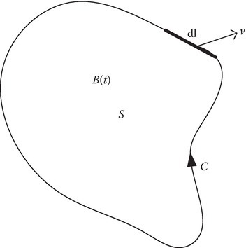
FIGURE 14.3
Geometry for Faraday’s law statement of (14.17).
The last term on the right-hand side (RHS) of (14.16) gives the total electromotive force (emf) induced in the closed circuit C, which could be changing with time, also the point function B could as well be changing with time. Equation 14.17 separates the contributions due to time-changing magnetic flux density field [called transformer emf, the first term on the RHS of (14.17)] and due to time-varying circuit C [motional emf, the second term on the RHS of (14.17)]. The last term on the RHS of (14.17) can be changed to . The term v × dl is the area swept by the element in 1 s. The last term is thus equal to −dΦm/dt due to the motion.
Applying Stoke’s theorem, the closed line integrals in (14.17) can be converted to surface integrals:
Since (14.18) is true for any S, provided it is the same S on all the integrals in (14.18), the integrands must be the same on both sides of (14.18).
Equation 14.18 is the same as (1.61) except that we used in (14.18) the symbol E′ instead of E to emphasize that the electric field in the definition of the emf for a moving circuit has to be the effective electric field. The expression for E′ can be obtained from (1.6) from its definition as the force for unit charge and is given by
Substitution of (14.20) in (14.19) results in (1.1), the differential form of Faraday’s law in the laboratory frame.
We can also show [10] that (14.20) and (14.22) are the consequence of imposing Galilean invariance of the form of Faraday’s law in differential form, that is,
Similarly, we can show [10] that the form invariance of Ampere’s law (1.2) under GT gives us the following additional relationships among the fields in inertial and laboratory frames:
There is some inconsistency among Equations 14.20 and 14.22, 14.23 and 14.24. For example, let us apply these equations to free space and show the inconsistency. From (14.20),
Equation 14.25 is in variance with (14.23).
Similarly, from (14.23),
Equation 14.26 is in variance with (14.22). Note that they become the same if c is taken as infinity. We have to reject the GT of Maxwell’s equations for moving media even for the nonrelativistic velocities of the medium. We show next that LTs given in the next section overcome these difficulties. For nonrelativistic velocities we can then formulate first-order Lorentz transformations (FOLT) as consistent approximations [4] discussed in Section 14.18.
GT does not alter the Newton’s force equation since
since
However, under LTs, to be discussed in the next section, we show that t ≠ t′, v ≠ v′ + v0, m ≠ m′, F ≠ F′, and that GT is valid only for nonrelativistic velocities. For arbitrary value of the parameter β = v0/c, one needs to consider relativistic mechanics based on LTs. LTs are connected with the theory of special relativity and a four-dimensional space.
14.4Lorentz Transformation
Since t = t′, in the GT, this transformation leaves the distance between two physical points unchanged in all coordinate systems.
The velocity of light as measured by a moving observer on z axis (at rest in ∑′) will be (c − v0) for the geometry shown in Figure 14.2. However, experiments show that the velocity of light as measured by a stationary observer or a moving observer will remain the same. This first postulate of the theory of special relativity is well confirmed. LTs in four-dimensional space x, y, z, ict will preserve the first postulate.
Let us, for convenience, use the nomenclature xμ, μ = 1, 2, 3, 4 to designate the coordinates in the four-dimensional space:
Note that we write the time component with the subscript 4 and designate it as imaginary. This should be carefully distinguished from [4] the imaginary notation in “quantum theory and wave theory” in some books. An alternative definition of x4 without i in its definition is discussed in Section 14.19.
The distance between two points in the four-dimensional space will remain the same provided
For the geometry shown in Figure 14.2,
Equation 14.36 will be satisfied if
Moreover, in the limit v0 → 0
The origin of ∑′ moves with a velocity v0 with respect to the origin ∑. Thus, we have the position of the origin of ∑′ as z = vt. Substituting z′ = 0 in (14.39),
Solving the relevant equations with signs chosen to agree with (14.42), we obtain
Thus, we have
where
Generalization of the above, where the relative velocity between ∑ and ∑′ is v0 instead of , is straightforward and is given by
Equation 14.50 can be written as
Equations 14.46 and 14.47 give rise to the length contraction and time dilation
In (14.52) [3] L = z2 – z1, where z2 and z1 are the instantaneous coordinates of the end points of the rod, observed at the same time t; , where and are the coordinates at the end points in ∑′.
Equation 14.53b [3] is interpreted as time dilation. A clock moving relative to an observer is found to run more slowly than one at rest relative to the observer. Considering unstable elementary particles as a clock, one can explain the time dilation concept by examining the lifetime of the particles. In (14.53), τ0 is the lifetime of the particle at rest in the system ∑′. The particle is moving with a uniform velocity v0 relative to the system ∑. When viewed from ∑, the moving particle lives longer than a particle at rest in ∑. The “clock” in motion is observed to run more slowly than an identical one at rest. Reference [2] has a number of graphs and examples to illustrate length contraction and time dilation.
14.5Lorentz Scalars, Vectors, and Tensors
Equation 14.36 is a constraint involved in the rotation of coordinates in the four-dimensional space. R is an invariant under LTs. LTs are rotations in a four-dimensional Euclidean space. This orthogonal transformation can be written as
For the geometry of Figure 14.2, the transformation matrix is given by
Figure 14.4a shows the geometry of rotation of the coordinates in the x3 – x4 plane by an angle ψ that achieves the LT.

FIGURE 14.4
Lorentz transformation: (a) rotation angle for the orthogonal transformation and (b) time dilation and the length contraction of the transformation.
An inverse transformation is obtained by reversing the sign of β, which gives aνμ. Thus we have
We also have
Equations 14.54a and 14.54b show that LT is an orthogonal transformation.
From the geometry (Figure 14.4), OC = OA + AC, giving
Similarly,
Comparing (14.56) with (14.54c), we get
Note that the angle ψ is complex and its cosine, cos ψ = γ ≥ 1. Thus, LT as a rotation, by an angle ψ, is a concept rather than a real angular rotation. Figure 14.4b shows L, L0, T, T0. The distance L0 in the frame ∑′ is observed as L in the frame ∑ at constant time in ∑. Though L appears larger than L0 in the figure, because of the complex nature of ψ,
The time interval T0 in the frame ∑′ is seen as T in the frame ∑, where
A quantity that does not change under LT is called a Lorentz scalar, say Φ. Its derivative (can be called four-gradient) with respect to is a four-vector.
The derivative transforms like a four-vector.
The four-divergence of a four-vector is Lorentz invariant:
If Aμ = ∂Φ/∂xμ, (14.61) shows that the four-dimensional Laplacian operator is a Lorentz invariant operator.
where ▫′ is the vector operator in four dimensions in (14.61) and ▫2 = ▫ ⋅ ▫ in (14.62).
The scalar product of two four-vectors is a scalar invariant
Lorentz scalar can be considered as a tensor of zero rank and four-vector as a tensor of rank one.
A second-rank tensor is a set of 16 quantities that transforms as
An example of such a tensor is the field strength four-tensor Fμν, which can be used to combine two of the Maxwell equations, as shown in the next section.
14.6Electromagnetic Equations in Four-Dimensional Space
In the four-dimensional space,
One can write the electromagnetic equations in terms of suitably chosen scalars, four-vectors, and four-tensors of second rank. The quantity in four-dimensional space will be denoted by an italic symbol with a subscript μ. Also a shorthand notation, that a repeated Greek letter subscript implies summation over that subscript as it varies from 1 to 4, will be used.
Let us start with the continuity equation (1.5)
Let
Equation 1.5 is
Since μ is a Greek symbol that is repeated, we can use the shorthand notation given as the last term in (14.67).
Moreover, if we definite the four-vector differential operator ▫
the continuity equation can be written, in terms of four divergence, as
where the bold italic Jμ is a four-vector current density.
Let us next consider the Lorentz condition, when the medium is free space, from (1.21):
Let us consider the four-vector potential Aμ:
Equation 14.71 can be written as
The wave equation in free space
can be written as
Note that (14.73b) is obtained from
If the source is a point charge Q moving with a relativistic velocity v along a specified trajectory, the scalar and vector potentials, called Lienard–Wiechert potentials, can be calculated and discussed in Appendix 14G. We touched on this topic in Chapter 13 also.
The field strength tensor Fμν can be constructed so that the equations
are satisfied. For example, from (14.75) and (14.76) we can write
If (14.75) and (14.76) can be written (in the form of a four-dimensional curl operation) as
then (14.77) is (14.78) with μ = 3, ν = 2, and Fμν = F32 = − B1 = − Bx.
One can verify that (14.75) and (14.76) become (14.78) if Fμν, a 4×4 matrix, has the following elements expressed in terms of the components of E and B.
Though we only verified the element F32 = − B1, one can check the correctness of the other elements.
With this field strength tensor, we can show that the two Maxwell equations in free space
take the form, in Lorentz space,
The two Maxwell equations, valid in any medium,
can be expressed in Lorentz space
For this reason Fμν is called field strength tensor. From (14.79), we note it is an antisymmetric tensor. The other two Maxwell equations, valid in any medium
can be combined as [10]
where
Since Gμν is a second-rank tensor, it transforms as
It is an antisymmetric tensor and can be called as excitation tensor.
14.7Lorentz Transformation of the Electromagnetic Fields
The field strength Fμν is a tensor; its transformation is given by (14.62).
The inverse transformation is obtained by interchanging primed and unprimed quantities and replacing β by −(β). For a general velocity υo, one can generalize (14.90)–(14.91) by
14.8Frequency Transformation and Phase Invariance
A four-vector wave number kμ can be constructed
so that
Since (14.93b) is a Lorenz scalar, it is Lorentz invariant giving the concept of phase invariance. Thus, we obtain (14.94)
Equation 14.94 leads to the results given by (14.95):
where θ and θ′ are the angles of k and k′ relative to the direction of υo. Equation 14.95a is the relativistic formula for the frequency shift, called relativistic Doppler effect. Equation 14.95b is the relativistic formula for aberration [4]. Equations 14.95 can be more easily seen by considering the motion of the frame to be on the z-direction, and the wave is propagating in the x–z plane.
Dividing (14.96b) by (14.96d), we obtain (14.95b).
From (14.94), we obtain
which is the same as (14.95a).
14.9Reflection from a Moving Medium
Let us solve the problem of determining the power reflection coefficient α of a moving medium. We will use the LT technique to solve the problem. The incident wave will be transformed to the primed frame in which the medium 2 is at rest, and this reflection problem in the rest frame with a stationary boundary can be solved using the techniques developed in Chapter 2. After obtaining the primed reflection coefficient R′, we will relate it to the unprimed R.
14.9.1Incident s-Wave
Let the s-wave in free space have the electric field
The ∑′ frame is attached to the moving conductor which is moving with a velocity
with reference to the laboratory frame ∑. The geometry is as shown in Figure 14.1.
We will transform the incident wave to ∑′ frame in which the moving conductor is at rest:
From the LT (14.96),
This leads to
where
where
The wave vector and the frequency of the reflected wave can be determined through (14.97).
From the phase invariance principle, the phase of the reflected wave as seen in ∑′ and ∑ are the same:
From (14.99), (14.46), (14.47), and (14.50),
Substituting (14.97) in (14.100), (14.101), (14.102), we obtain the following:
where
As an aside, let us list the results for the case of the medium moving with velocity vo along x-axis, , and we obtain the following (the student is advised to derive these equations):
where
14.9.2Field Transformations
In ∑′ the medium is stationary, and can be calculated using the theories developed for the stationary media. The electromagnetic properties of the medium 2 in ∑′ determine . For example, if the medium 2 is a perfect electric conductor .
The relation between and Rs, where
can be obtained from LT (14.92) for the fields. For the case of ,
Dividing (14.107b) by (14.107a), we obtain
It can be noted that the factor in the brackets () in (14.108) comes from the transformation of fields in the incident medium, depending on the velocity of the moving second medium and the angle of incidence. It is not influenced by the properties of medium 2.
14.9.3Power Reflection Coefficient of a Moving Mirror for s-Wave Incidence
If the medium 2 is a PEC, , and the power reflection coefficient α is given by
Simplifying (14.109b), the power reflection coefficient for the case of s-wave incidence on a PEC moving perpendicular to the interface is given by
It is worth remarking that the PEC medium is a perfect reflector and α is the highest power reflection coefficient that can be achieved by any second medium. If the second medium is not a perfect reflector, for example, if the second medium is a dielectric or a plasma, certain amount of power can be transmitted into the second medium and will not be one. However, the power reflection coefficient ρ can be expressed for such a case as α times
Figure 14.5 shows the plot of α vs. β. The parameter C = 0.5, that is, the angle of incidence θ = 60°. The angle of reflection θ′ as seen in ∑′ and the angle of reflection θr as seen in ∑ are also shown.

FIGURE 14.5
The power reflection coefficient α, the angle of reflection θ′ as seen in ∑′, and the angle of reflection θr as seen in ∑ as a function of β are shown. The angle of incidence θ = 60°, given C = cos θ = 0.5. α scale is logarithmic. Note that α > 1 for β < 0. Also note that , where S = sin θ.
Several interesting points can be noted from Figure 14.5. α is zero at , since the angle of reflection θr, as seen in ∑, is 90° at this value of β. In the range , θr > 90° and α is thus negative.
This means that in this range of β, the reflected wave travels towards the medium 2 as seen from ∑. For an interpretation of Figure 14.5, for the range C < β < 1, see [12], which is given as Appendix 14A.
Another surprising result is that α is greater than one for the range of −1 < β < 0. This phenomenon can be explained by noting that mechanical power is supplied to the system to maintain the uniform motion of the conductor against the radiation pressure. A detailed calculation of the electric power Pel, the rate of the decrease of the stored energy in the fields Ps, and the mechanical power supplied to the medium to overcome the radiation pressure force Pm for the conductor as well as the dielectric half-space are given in Appendix 14B [23].
This appendix contains many more references on the topic.
14.10Constitutive Relations for a Moving Dielectric
Minkowsky theory is developed based on
for a simple loss-free medium, where ε′ and μ′ are the parameters measured in ∑′. Using field transformations, one can obtain the constitutive relations of the Minkowsky theory.
Equations 14.113 and 14.114 are obtained using (14.92) and (14.115):
Equations 14.115 are obtained from (14.85) [10].
The constitutive relations in ∑ can now be written as [6]
where
In the above, it is assumed that .
14.11Relativistic Particle Dynamics
A brief review of the relativistic particle dynamics is given below. A more complete account can be found in [3]. The charge of an electron q is invariant. However, the mass of an electron m is given by
where mo is the rest mass.
The relativistic momentum of a mass m moving with velocity vo
In a collision it is this momentum that is conserved and not the classical momentum mvo. The relativistic force
The four momentum of a particle of energy
transforms as a four-vector, giving
Given
The inverse transformation can be obtained by changing β → − β and interchanging the primed and unprimed quantities.
In the above, ∑′ is moving in the direction of z = x3. The length of the four-vector pu is a scalar invariant:
In the rest frame of the particle, p′ = 0, and we get the equation
If the particle is moving along z-axis
then
Equation 14.130 can be interpreted as a relationship between three sides of a right-angled triangle. The hypotenuse is the relativistic energy and of the two sides making the right angle, one of them is the rest energy moc2 [1].
The total energy ε is the sum of the rest energy moc2 and the kinetic energy T given by
To summarize, a free particle with rest mass mo moving with a velocity vo in a reference frame Σ has a momentum p and energy given by
A photon in free space has an energy :
where h is Plank’s constant and f is the frequency in Hz, ℏ = h/2π, and ω is the frequency in radians/s.
Its velocity is c. Its momentum is given by
14.12Transformation of Plasma Parameters
The plasma frequency in the respective frames are given by
where (−q′, m′, N′) and (−q, m, N) are the electron charge, mass, and volume electron number density in their respective frames.
Since
we obtain
Thus,
14.13Reflection by a Moving Plasma Slab
In Section 14.9, we discussed the key steps in solving the moving media problem. The first step is to obtain the reflection coefficient R′ in the rest frame. The second step is to relate the reflection coefficient R′ to R by considering the transformation of the fields and reflection angle in the laboratory frame and to determine the factor α, which was identified as the power reflection coefficient of a moving mirror. The power reflection coefficient ρ for any moving, transmitting medium can then be expressed as
In Section 14.9 we showed, for s-wave and the mirror movement perpendicular to the interface,
and the power reflection coefficient for the moving mirror
It can be shown that for p-wave
where
Substituting for the p-wave incidence on a mirror in (14.147), the power reflection coefficient when the mirror is moving perpendicular to the interface is given by
On simplification, (14.148) will be the same as (14.146).
Appendix 14A discusses the isotropic moving plasma slab problem by computing . Section 9.4 also deals with the stationary plasma slab problem. Appendix 14C [14] discusses the uniaxial plasma slab problem with
where is given by (14.143).
14.14Brewster Angle and Critical Angle for Moving Plasma Medium
Appendix 14D [18] discusses the Brewster angle for a plasma medium moving at a relativistic speed. Appendix 14E [22] discusses the total reflection of electromagnetic waves from moving plasmas.
14.15Bounded Plasmas Moving Perpendicular to the Plane of Incidence
Appendix 14F [20] discusses the reflection properties of a plasma moving perpendicular to the plane of incidence. This reference is included in this book as Appendix 14F.
14.16Waveguide Modes of Moving Plasmas
References 11,16,17,19,21,28, and 29 discuss the waveguide modes of moving plasmas.
14.17Impulse Response of a Moving Plasma Medium
References 24,25,26 and 30 discuss the reflection of an impulse plane wave by moving plasma half-spaces.
14.18First-Order Lorentz Transformation
One is tempted to use the GT for nonrelativistic velocities. However, we have shown in Section 14.3 that such an attempt can lead to inconsistent approximations. Since Maxwell’s equations are covariant with LTs, the best way to solve a moving media electromagnetic problem is to solve the problem using LTs, and for nonrelativistic velocities, drop the terms of the order of β2 and higher. The resulting transformations are called [4] FOLT. In FOLT, γ is approximated by one. Listed below are the FOLT approximations of some of the equations given earlier using LT.
| LT | FOLT |
|---|---|
|
(14.46)
|
(14.46F)
|
|
(14.47)
|
(14.47F)
|
|
(14.92b)
|
(14.92bF)
|
It can be noted that one can obtain GT as an approximation of LT if the limit c approaches infinity rather than ignoring terms of β2 and higher for nonrelativistic velocities involved in applying FOLT. This explains the inconsistencies that arise in using GT for electromagnetic problems.
14.19Alternate Form of Position Four-Vector
As mentioned in Section 14.5, L appears larger than L0 and T appears smaller than T0 in Figure 14.4b, since the rotation angle ψ is complex. In some books, for example [1], alternative definitions of the position four-vector and its norm are used as given below:
Note the negative sign before in the middle term of (14.151). The norm in this case in not the distance in four-dimensional space-time in the sense of Euclidean geometry. In the previous definition of the fourth component of the position four-vector given in (14.65), the multiplier i appears before ct, making ψ complex. However, the norm, as defined by R according to (14.36), is the distance in the Euclidean sense in the four-dimensional space-time. A geometrical picture of the LT with the new definition of the four-vector and its norm given in (14.150) and (14.151), respectively, is shown in Figure 14.6.
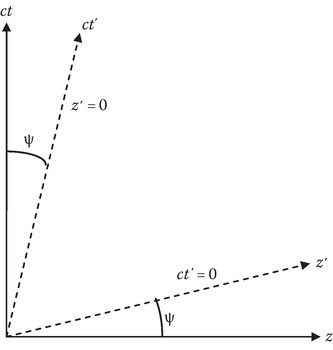
FIGURE 14.6
A geometrical picture of the LT with the new definition of the four-vector and its norm given in (14.150) and (14.151), respectively.
It is called Minkowski diagram. Compare it with Figure 14.4 a. One of the problems at the end of the chapter brings out the advantages of Minkowski diagram in visualizing the concepts of length contraction and time dilation.
Given below are the changes in the form of some of the equations in the previous sections adapted to the choice of position four-vector (14.150) and the norm (14.151). The equation numbering used for these equations has the last character as n, to make it easy to compare with the corresponding equation in the previous sections:
As far as the case of a medium moving uniformly with the velocity v0, special relativity applies and the choice of (a) position four-vector as in (14.65) with the associated norm as the Euclidean distance in four dimensions or (b) position four-vector as defined in (14.150) and its norm as defined in (14.151) is a “matter of taste” [5]. The author has chosen (a).
When the medium is accelerating, general relativity applies, and there are some advantages in choosing the alternative notation given in (b). The calculations will be much facilitated by invoking additional concepts of tensors with covariant and contravariant components, the summation convention, etc. Reference [5] deals with such applications.
References
- 1.Lorrain, P., Corson, D.P., and Lorrain, F., Electromagnetic Fields and Waves, 3rd edn., W.H. Freeman and Company, New York, 1988.
- 2.Schmitt, R., Electromagnetics Explained, Newnes, and Imprint of Elsevier Science, Boston, MA, 2002.
- 3.Jackson, J.D., Classical Electrodynamics, John Wiley, New York, 1962.
- 4.Kong, J.U., Electromagnetics Wave Theory, EMW Publishing, Cambridge, MA, 2002.
- 5.Van Bladel, J., Relativity and Engineering, Springer-Verlag, New York, 1984.
- 6.Chawla, B.R. and Unz, H., Electromagnetic Waves in Moving Magneto-Plasmas, The University Press of Kansas, Lawrence/Manhattan/Wichita, 1971.
- 7.Shrivastava, R.K., The interaction of electromagnetic waves with relativistically moving bounded plasmas, Doctoral thesis, Birla Institute of Technology, Ranchi, India, 1975.
- 8.Prasad, R.C., Transient and frequency response of a bounded plasma, Doctoral thesis, Birla Institute of Technology, Ranchi, India, 1976.
- 9.Prasad, R., Wave propagation in plasma waveguides and experimental simulation, Doctoral thesis, Birla Institute of Technology, Ranchi, India, 1979.
- 10.Papas, C.H., Theory of Electromagnetic Wave Propagation, McGraw-Hill, New York, 1965.
- 11.Kalluri, D., Waveguide modes of a warm drifting unaxial electron plasma, Proc.IEEE, 58(2), 278–280, 1970.
- 12.Kalluri, D. and Shrivastava, R.K., Electromagnetic wave interaction with moving bounded plasmas, J.Appl.Phys., 44(10), 4518–4521, 1973.
- 13.Kalluri, D. and Shrivastava, R.K., Reflection and transmission of electromagnetic waves obliquely incident on a relativistically moving isotropic plasma slab, J.Appl. Phys., 44(5), 2440–2442, 1973.
- 14.Kalluri, D. and Shrivastava, R.K., Reflection and transmission of electromagnetic waves obliquely incident on a relativistically moving unaxial plasma slab, IEEE Trans. Antennas Propag., AP-21(1), 63–70, 1973.
- 15.Kalluri, D. and Shrivastava, R.K., On reflection and transmission of electromagnetic waves obliquely incident on a relativistically moving unaxial and isotropic plasma slab, IEEE Trans. Plasma Sci., PS-2, 206–210, 1974.
- 16.Kalluri, D. and Prasad, R., Comments on characteristics of waveguides filled with homogeneous lossy anisotropic drifting plasma, Int.J. Electron. (England), 38(4), 573–574, 1975.
- 17.Kalluri, D. and Prasad, R., Waveguide modes of a warm unaxial lossy drifting electron plasma, Int.J. Electron. (England), 39(6), 637–646, 1975.
- 18.Kalluri, D. and Shrivastava, R.K., Brewster angle for a plasma medium moving at relativistic speed, J. Appl. Phys., 46(3), 1408–1409, 1975.
- 19.Kalluri, D., Waveguide modes of a warm drifting unaxial electron plasma for large drifting velocities, IEEE Trans.Antenna Propag., AP-23(5), 745, 1975.
- 20.Kalluri, D. and Prasad, R.C., Interaction of electromagnetic waves with bounded plasmas moving perpendicular to the plane of incidence, Appl. Phys., 48(2), 587–591, 1977.
- 21.Kalluri, D. and Prasad, R., Waveguide modes of a warm unaxial lossy drifting electron plasma for large drift velocities, IEEE Trans.Plasma Sci., PS-6(4), 593–598, 1978.
- 22.Kalluri, D. and Shrivastava, R.K., On total reflection of electromagnetic waves from moving plasmas, J. Appl. Phys., 49(12), 6169–6170, 1978.
- 23.Kalluri, D. and Shrivastava, R.K., Radiation pressure due to plane electromagnetic waves obliquely incident on moving media, J. Appl. Phys., 49(6), 3584–3586, 1978.
- 24.Kalluri, D. and Prasad, R.C., Reflection of an impulsive plane wave by a plasma half-space moving perpendicular to the plane of incidence, J. Appl, Phys., 49(5), 2696–2699, 1978.
- 25.Kalluri, D. and Prasad, R.C., On impulse response of plasma half-space moving normal to the interface-II: Results, 1979 IEEE International Conference on Plasma Science, Montreal, Quebec, Canada, Conference Record-Abstracts, pp. 154–155, June 4–6, 1979.
- 26.Kalluri, D. and Prasad, R.C., On impulse response of plasma half-space moving normal to the interface-I: Formulation of the solution, 1979 IEEE International Conference on Plasma Science, Montreal, Quebec, Canada, Conference Record-Abstracts, p. 155, June 4–6, 1979.
- 27.Shrivastava, R.K. and Kalluri, D., On brewster angles for perpendicularly polarized electromagnetic waves interacting with a moving dielectric half-space, Proceedings of the Symposium on “Topics in Applied Physics”, Calcutta University, Kolkata, India, February 1979.
- 28.Kalluri, D. and Prasad, R., Waveguide modes of a warm transversely drifting electron plasma with strong transverse magnetic field, IEEE Trans.Plasma Sci., PS-7(1), 6–9, 1979.
- 29.Kalluri, D. and Prasad, R., Waveguide modes of a warm isotropic drifting electron plasma, J.Appl. Phys., 50(4), 2675–2677, 1979.
- 30.Prasad, R.C. and Kalluri, D., Impulse response of a lossy magnetoplasma half-space moving along the magnetic field, 1980 IEEE International Conference on Plasma Science, Madison, WI, Conference Record-Abstracts, pp. 11–12, May 1921, 1980.