Search in book...
Toggle Font Controls
Create new playlist

Name your new playlist

Playlist description (optional)
Sign In

Email address

Password

Forgot Password?

or

Continue with Facebook

Continue with Google
Sign Up

Full Name

Email address

Confirm Email Address

Password

or

Continue with Facebook

Continue with Google

Time-Domain Solutions

13
Time-Domain Solutions

13.1Introduction

Section 1.3 briefly dealt with the solution of Maxwell’s equations in time domain. A simple example of obtaining the radiated fields when a point electric dipole is excited by an impulse current was discussed. Most of the rest of the chapters till now dealt with time-harmonic fields using the concept of phasors. We assumed that the transient response when needed can be obtained from the frequency response using a superposition integral. Using the Laplace transform technique and replacing (jω) by the Laplace transform variable s in the frequency response, we obtained the impulse response of a plasma half-space when excited by an impulse s wave in Section 9.9.

In this chapter, we will explore in a systematic way the direct solution of the Maxwell’s equations in the time domain. Let us begin with the solution of the one-dimensional scalar wave equation for the scalar potential ψ(z, t) in free space given by (1B.38) and repeated here as (13.1):

(13.1)

$\frac{\partial^{2} ψ (z, t)}{\partial z^{2}} - \frac{1}{c^{2}} \frac{\partial^{2} ψ (z, t)}{\partial t^{2}} = 0.$

With zero initial conditions, we showed that the scalar potential is given by (1B.43) and repeated here as (13.2):

(13.2)

$ψ (z, t) = f_{1} (t - \frac{z}{c}) + f_{2} (t + \frac{z}{c}) .$

The functions f₁(t) and f₂(t) will be determined by the two boundary conditions needed to solve the second-order partial differential equation (PDE) (13.1). We illustrated through Figure 1B.4 that the first term on the right-hand side (RHS) of (13.2) is a forward-going impulse wave traveling with a velocity c in the positive z-direction, if f₁(t) is an impulse δ(t). The voltage of an ideal transmission line satisfies a wave equation similar to (13.1) and is given by (2.52). In the next section, we will exploit the interpretation of the solution (13.2) to study the propagation of pulses on a bounded transmission line excited at the left end of the line and loaded at the right end.

13.2Transients on Bounded Ideal Transmission Lines

Figure 13.1 shows an ideal transmission line, excited by a source at the source end z = 0, which is switched on at t = 0. The source is modeled by an ideal voltage source whose internal impedance is R_g. The z = l is the load end of the transmission line and R_L is the load resistance.

FIGURE 13.1
Geometry to study the transients on a transmission line.

The wave equation for voltage V(z, t) of the ideal transmission line is given by (2.52). Figure 13.1 is the modified version of Figure 2.5, modified to study the propagation of transient waves on ideal transmission lines as opposed to the steady-state analysis of Section 2.8. The solution can be written as

(13.3)

$V (z, t) = V^{+} (t - \frac{z}{v}) + V^{-} (t + \frac{z}{v}),$

where v is given by (2.53). It can be shown from (2.51) that the current I(z, t), with G′ = 0, is given by

(13.4)

$I (z, t) = I^{+} (t - \frac{z}{v}) + I^{-} (t + \frac{z}{v}) = \frac{1}{Z_{0}} [V^{+} (t - \frac{z}{v}) - V^{-} (t + \frac{z}{v})],$

where, with R′ = 0,

(13.5)

$Z_{0} = \frac{1}{C^{'} v} = \sqrt{\frac{L^{'}}{C^{'}}} .$

Note the negative sign in front of the last term in (13.4), giving the correct sign for the power VI in the negative-going wave. To summarize,

(13.6)

$V^{+} (z, t) = Z_{0} I^{+} (z, t)$

(13.7)

$V^{-} (z, t) = - Z_{0} I^{-} (z, t) .$

13.2.1Step Response for Resistive Terminations

Several examples follow to illustrate as well as establish the well-known techniques of bookkeeping of the effect of reflections of the waves at the source end and the load end. However, it is instructive to have a qualitative discussion of the broad principles that govern the transient response of bounded transmission line problem as given in Figure 13.1. For the purpose of this qualitative discussion, let us assume that the source is a battery of voltage V₀ and the transmission line is uncharged with both voltage and current zero for t = 0⁻. When the switch is closed at t = 0, the source end S will be immediately, at t = 0⁺, excited with a step function, that is, V(0, 0⁺)= Au(t). The amplitude A has to be determined taking into account the effect of R_g. Since the excited positive-going wave V⁺(z, t) travels with a finite velocity and the line is uncharged, it only sees the impedance Z₀, and the current I⁺(z, t) will be V_g/(R_g + Z₀) and A = V_g Z₀/(R_g + Z₀). Thus, a positive-going wave Au(t − z/v) is launched on the line. When this wave reaches the load end in a period T = l/v, it encounters the lumped element load with a specified voltage–current relationship, which may not be satisfied by the voltage–current relationship of the positive-going wave. We can consider the positive-going wave as the incident wave at the load end. This imbalance is resolved by superposition of a suitable negative-going wave V⁻(z, t), which we can call as reflected wave at the load. The ratio of the voltage of the reflected wave to that of the incident wave at the load end can be defined as $Γ_{L}^{V}$ . Similar ratio for currents, defined as $Γ_{L}^{I}$ , can easily be shown to be the negative of $Γ_{L}^{V}$ . At t = 2T, the wave reaches the source end S. Now the negative-going wave becomes the incident wave at the source end, and to satisfy the voltage–current relationship at the source end, another positive-going wave will be generated. The parameters $Γ_{S}^{V}$ and $Γ_{S}^{I}$ will relate the voltage and current of the newly generated positive-going wave. This process of bouncing of waves at both the ends describes qualitatively the successive generation and traveling of the positive-going and negative-going waves on the bounded transmission line. The expressions for the reflection coefficients described above can be obtained from the boundary conditions as given below.

At the load end L,

(13.8)

$R_{L} I_{L} (t) = V_{L} (t)$

(13.9)

$\frac{R_{L}}{Z_{0}} [V^{+} (l, t) - V^{-} (l, t)] = [V^{+} (l, t) + V^{-} (l, t)] .$

From (13.8) and (13.9), the expressions for the reflection coefficients can be obtained:

(13.10)

$Γ_{L}^{V} = \frac{V^{-} (l, t)}{V^{+} (l, t)} = \frac{R_{L} - Z_{0}}{R_{L} + Z_{0}}$

(13.11)

$Γ_{L}^{I} = \frac{I^{-} (l, t)}{I^{+} (l, t)} = \frac{V^{-} (l, t) / (- Z_{0})}{V^{+} (l, t) / (Z_{0})} = - Γ_{L}^{V} .$

At the source end S,

(13.12)

$V_{s} (t) = V_{g} (t) - R_{g} I_{s} (t) = V^{+} (0, t) + V^{-} (0, t)$

(13.13)

$I_{s} (t) = [I^{+} (0, t) + I^{-} (0, t)] = \frac{1}{Z_{0}} [V^{+} (0, t) - V^{-} (0, t)] .$

Solving for V⁺(0, t),

(13.14)

$V^{+} (0, t) = \frac{Z_{0}}{R_{g} + Z_{0}} V_{g} (t) + \frac{R_{g} - Z_{0}}{R_{g} + Z_{0}} V^{-} (0, t) .$

The first term on the RHS of (13.14) can be identified with the amplitude A of the unit step mentioned above and the coefficient of the second term on the RHS of (13.14) with $Γ_{s}^{V}$ :

(13.15)

$Γ_{s}^{V} = \frac{R_{g} - Z_{0}}{R_{g} + Z_{0}} .$

These definitions of the reflection coefficients in the time domain are in line with our understanding of the definitions of the reflection coefficients in Section 2.8. The source end definitions are in accordance with Thevenin’s theorem.

A bounce diagram, shown in Figure 13.2, is a useful technique to keep track of effects of the successive reflections from the load and source ends. The horizontal axis is the z-axis and the vertical axis is the t-axis. At t = 0⁺, a positive-going step wave of voltage function $V_{1}^{+}$ of amplitude A is launched, and it travels on the line with a velocity v as shown by the straight line with a slope v. It reaches the load end L in a time period T = l/v. It is this incident wave that encounters the impedance mismatch and gives rise to a reflected wave whose voltage is denoted by $V_{1}^{-} = Γ_{L}^{V} V_{1}^{+}$ . At t = 2T, this wave reaches the source end and will be reflected at the source end giving rise to $V_{2}^{+} = Γ_{L}^{V} Γ_{S}^{V} V_{1}^{+}$ . At t = 3T, a second reflection takes place at the load end giving rise to $V_{2}^{-} = Γ_{L}^{V} {(Γ_{L}^{V})}^{2} V_{1}^{+}$ .

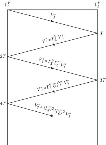
FIGURE 13.2
Bounce diagram of successive reflections.

The voltages of the successive reflected waves at the source and load ends are as shown in Figure 13.2. It is now easy to show [1] that

(13.16)

$V (z, \infty) = V_{1}^{+} \frac{1 + Γ_{L}^{V}}{1 - Γ_{L}^{V} Γ_{S}^{V}} .$

From (13.10), (13.15), and the expression for $V_{1}^{+} = A = \frac{Z_{0}}{R_{g} + Z_{0}} V_{g} (t)$ , we obtain

(13.17)

$V (z, \infty) = V_{g} \frac{R_{L}}{R_{g} + R_{L}} .$

Equation 13.17 confirms that in steady state, the voltage on the transmission line at any z is the same as the voltage drop across the load resistance, as expected when the source is a DC voltage V_g and the transmission line acts merely as connecting wire.

A bounce diagram for the current can be drawn on similar lines as above using the current reflection coefficients instead of the voltage reflection coefficients. From (13.11), the current reflection coefficient at the load end L is the negative of the voltage reflection coefficient. Similar statement is also true for the source end.

An alternative to the bounce diagram is a graphical method called Bergeron diagram [2,3,4], to represent the effects of successive reflections. Bergeron diagram is not that useful for linear loads and sources but is the best way to treat nonlinear loads and sources. However, its explanation is facilitated by looking at linear loads and sources. Figure 13.3 shows the relevant graphs for the linear case.

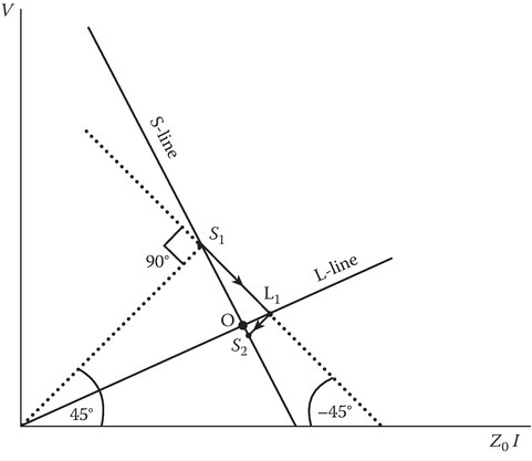
FIGURE 13.3
Bergeron diagram for a linear load.

The horizontal axis is a quantity proportional to the current and labeled as Z₀I. The vertical axis is the voltage. The two solid lines marked as S (source end) line and L (load end) line are the linear equations relating the V–I relationships at S and L points on the transmission lines. The operating point (intersection point of these two straight lines) represents the voltage, and current on the line in the limit t approaches infinity, when the interconnects (transmission line) act merely as connecting wires. However, the operating point is reached by successive reflections at the source and load ends.

The point S₁ applicable at t = 0 is the intersection of the S-solid line with the dotted 45^° line starting from the origin. The equations are

(13.18)

$V_{S} = V_{g} - \frac{R_{g}}{Z_{0}} (Z_{0} I_{S}) S — solid line$

(13.19)

$V^{+} = Z_{0} I^{+} 45^{°} line .$

The point L₁ applicable at t = T is located as the intersection of the two lines with the following two equations:

(13.20)

$V_{L} = \frac{R_{L}}{Z_{0}} (Z_{0} I_{S}) L — solid line$

(13.21)

$V^{-} = - Z_{0} I^{-} - 45^{°} line .$

The broken straight line S₁L₁ in Figure 13.3 is drawn from S₁ and continuing at −45^° till we reach the intersection point L₁ on the solid L-line. We next draw L₂S₂ at 45^° starting from L₁ and ending at S₂ on the S-solid line. Point S₂ represents the voltage–current relationship at t = 2T. We continue this process of locating L₂, S₃, L₃, etc., till we reach the operating point within a prescribed error or reach the limitation of the accuracy of the graphical method.

Some numerical examples are given below. In these examples, T = l/v.

Example 13.1

In Figure 13.1, assume R_g = 75 ohms (Ω), R_L = 100 Ω, and the source is a step voltage of 100 V. Let the length of the line l be 10 cm and the velocity of the traveling waves on the line as 2/3c, where c is the velocity of light. Let Z₀ be 50 Ω. Let the initial conditions on the transmission line be zero. Sketch V(0.25l, t).

Solution

We calculated T = 0.5 ns, $Γ_{S}^{V} = 1 / 5$ , $Γ_{L}^{V} = 1 / 3$ . We can now fill in the bounce diagram with numbers using the formulas developed above.

$V_{1}^{+} = 40$ , $V_{1}^{-} = 40 / 3$ , $V_{2}^{+} = 8 / 3$ , $V_{2}^{-} = 8 / 9$ , $V_{3}^{+} = 8 / 45$ , … V(z, ∞) = 400/7 = 57.07 V. From the bounce diagram, we can sketch V(0.25l, t) versus t as shown in Figure 13.4 and it reaches 56 at t = 9T/4, that is t = 1.125 ns. If we continue to graph further, the voltage will reach the asymptotic value of 57.07 V.

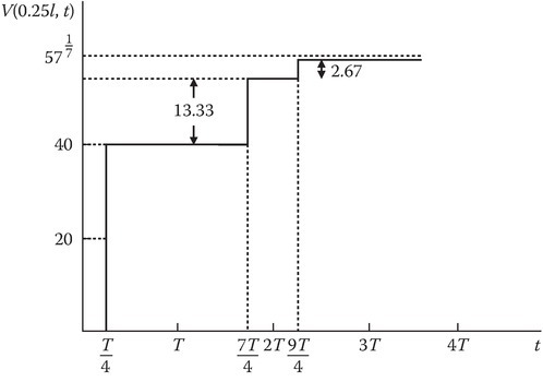
FIGURE 13.4
Sketch of the voltage V(0.25l, t) for the data of Example 13.1.

Example 13.2

Assume the same data as for Example 13.1 except R_L = Z₀ = 50 Ω. Load end is matched to the line. Sketch V(0.25l, t) and I(0.25l, t).

Solution

$V_{1}^{+} = 40 V, Γ_{L}^{V} = 0, V_{1}^{-} = 0,$

$I_{1}^{+} = 0.8 A, Γ_{L}^{I} = 0.$

$V (0.25 l, \infty) = 40 V, I (0.25 l, \infty) = 0.8 A .$

The sketches V(0.25l, t) and I(0.25l, t) are shown in Figure 13.5.

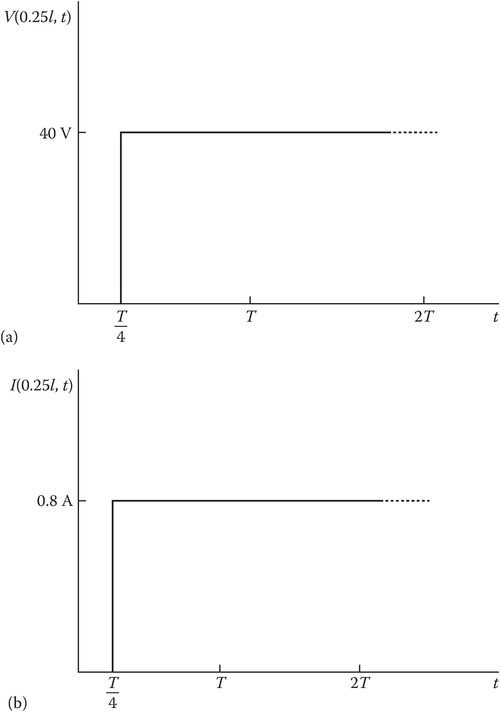
FIGURE 13.5
Sketches of (a) voltage and (b) current at *z = l/*4 for the data of Example 13.2.

Example 13.3

Assume the same data as for Example 13.1 except R_g = Z₀ = 50 Ω. The source end is matched to the line. Sketch V(0.25l, t) and I(0.25l, t).

Solution

$V_{1}^{+} = 50, Γ_{L}^{V} = 1 / 3, V_{1}^{-} = 50 / 3, Γ_{S}^{V} = 0, V_{2}^{+} = 0,$

$I_{1}^{+} = 1 A, Γ_{L}^{I} = - 1 / 3, I_{1}^{-} = 1 / 3 A, Γ_{S}^{I} = 0, I_{2}^{+} = 0$

$V (z, \infty) = 200 / 3 V, I (z, \infty) = 2 / 3 A .$

The sketches V(0.25l, t) and I(0.25l, t) are shown in Figure 13.6.

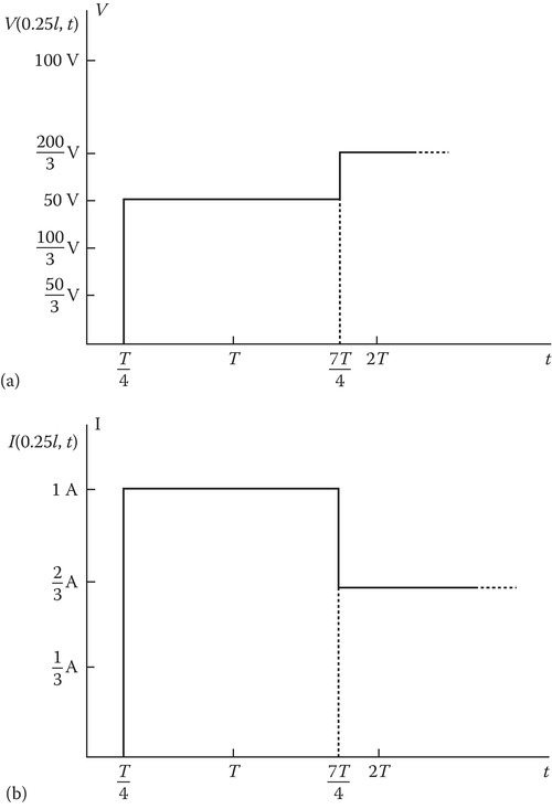
FIGURE 13.6
Sketches of (a) voltage and (b) current at *z = l/*4 for the data of Example 13.3.

Example 13.4

Assume the same data as for Example 13.1 except R_S = Z₀ = R_L = 50 Ω. The source end as well as the load end is matched to the line. Sketch V(0.25l, t) and I(0.25l,t).

Solution

$V_{1}^{+} = 50 V, Γ_{L}^{V} = 0, V_{1}^{-} = 0$

$I_{1}^{+} = 1 A, Γ_{L}^{I} = 0, I_{1}^{-} = 0$

$V (z, \infty) = 50 V, I (z, \infty) = 1 A .$

The sketches V(0.25l, t) and I(0.25l, t) are shown in Figure 13.7.

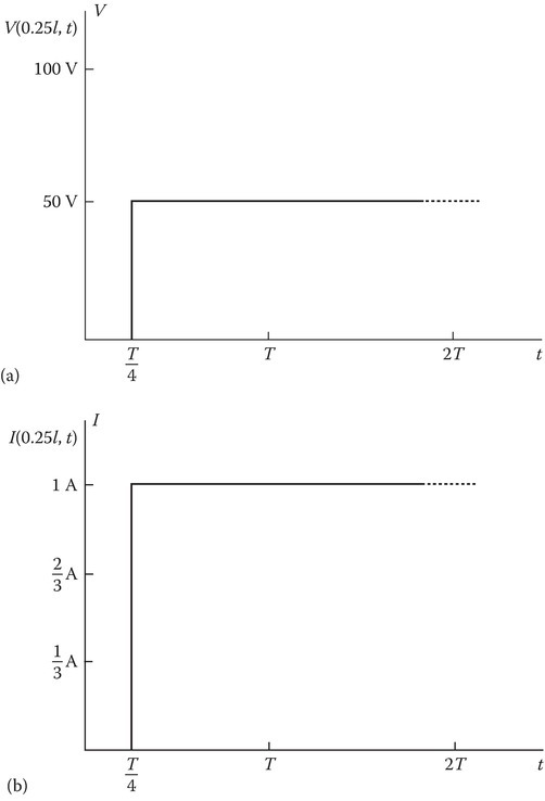
FIGURE 13.7
Sketches of (a) voltage and (b) current at *z = l/*4 for the data of Example 13.4.

Example 13.5

Assume the same data as for Example 13.3 except that R_L = ∞. Sketch V(0, t) and I(0, t).

Solution

$V_{1}^{+} = 50 V, Γ_{L}^{V} = 1, V_{1}^{-} = 50 V, Γ_{S}^{V} = 0, V_{2}^{+} = 0$

$I_{1}^{+} = 1 A, Γ_{L}^{1} = - 1, I_{1}^{-} = - 1 A, Γ_{S}^{I} = 0, I_{2}^{+} = 0$

$V (z, \infty) = 100 V, I (z, \infty) = 0.$

The sketches V(0, t) and I(0, t) are shown in Figure 13.8.

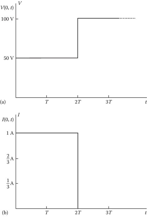
FIGURE 13.8
Sketches of (a) voltage and (b) current at *z =* 0 for the data of Example 13.5. At the load end, there is an open circuit.

Example 13.6

Assume the same data as for Example 13.3 except that R_L = 0. Sketch V(0, t) and I(0, t).

Solution

$V_{1}^{+} = 50 V, Γ_{L}^{V} = - 1, V_{1}^{-} = - 50 V, Γ_{S}^{V} = 0, V_{2}^{+} = 0$

$I_{1}^{+} = 1 A, Γ_{L}^{I} = 1, I_{1}^{-} = 1 A, Γ_{S}^{I} = 0, I_{2}^{+} = 0$

$V (z, \infty) = 0, I (z, \infty) = 2.$

The sketches V(0, t) and I(0, t) are shown in Figure 13.9.

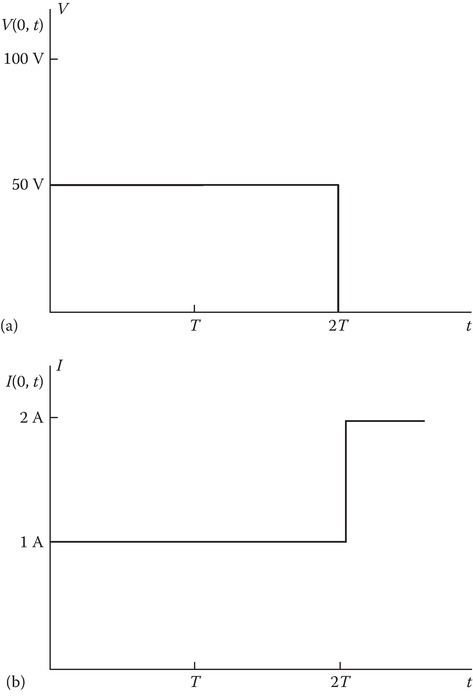
FIGURE 13.9
Sketches of (a) voltage and (b) current at source end for the data of Example 13.6. The source end is matched to the line but the load end is shorted.

Example 13.7

Assume the data of Example 13.4 of a transmission line matched at the source as well as the load end. However, in this example, we will consider the effect of a fault, represented by a parallel fault resistance R_f of unknown value, on the line at an unknown distance d from the source end. The sketch of the voltage V(0, t) is as given in Figure 13.10. Determine d and R_f.

Solution

From Figure 13.10, we note that the change in the voltage at the source end occurs at t = T/3, which is the delay time for the signal to travel from the source to the fault and the reflected wave generated at the fault to travel from the fault to the source end. Hence,

$2 d / v = T / 3 = (l / v) / 3$

$d = l/ 6.$

At z = d, $Γ_{f}^{V} = - (50 - 20) / 50 = - 3 / 5 = (Z_{d} - Z_{0}) / (Z_{d} + Z_{0})$ , solving which we get Z_d = (1/4)Z₀.

Since Z_d is the impedance of the parallel combination of R_f and Z₀,

(R_f Z₀)/(R_f + Z₀) = Z₀/4, solving which we get R_f = Z₀/3 = 50/3 Ω.

FIGURE 13.10
Voltage at the sending end for the data of Example 13.7. The line is matched to the load as well as the source, but a fault occurs at an unknown location.

13.2.2Response to a Rectangular Pulse

A rectangular pulse can be considered as the superposition of a unit step function with the negative of a delayed unit step function. Let us assume that the source voltage in Figure 13.1 is given by

(13.22)

$V_{g} (t) = u (t) - u (t - t_{s}) .$

One can draw two bounce diagrams for each of the sources u(t) and u(t − ts) and obtain the voltage at any point on the line as a function of time by appropriately combining the bounce diagrams. If the line is matched at the source end as well as the load end, the rectangular pulse of half the amplitude will be delivered to the load. There will be no further reflections, since the reflection coefficients at both the ends are zero.

13.2.3Response to a Pulse with a Rise Time and Fall Time

If the line is matched at both the ends appropriately, the pulse will be delivered faithfully to the load. However, if in addition to the load resistance of Z₀, the load terminals might give rise to parasitic capacitance in parallel with Z₀. In this case, the pulse will be distorted. One can study the effect of the capacitance on the voltage at the source end as well as the load end. We will give next an example simplifying the problem by assuming that the source is a step-like function with a ramp transition [4] defined in the example. We will use the Laplace transform technique.

13.2.4Source with Rise Time: Response to Reactive Load Terminations

To illustrate the effect of the rise time and parasitic capacitance at the load terminal, we will consider the following example.

Example 13.8

Assume the data of Example 13.4 of a transmission line matched at the source as well as the load end. However, we will make two changes: (a) The source is a step-like function with a ramp transition shown in Figure 13.11, defined as follows:

$V_{g} (t) = 0, t < 0$

(13.23)

$V_{g} (t) = t / a, 0 < t < a$

$V_{g} (t) = 1, t > a .$

The load is a parallel combination of Z₀ and capacitance C_L.

Solve analytically using the Laplace transform technique and also sketch the voltage waveform at the load end L and source end S.

Solution

The load Z_L(s), which is a parallel combination of Z₀ and 1/C_Ls, can be written as

(13.24)

$Z_{L} (s) = \frac{Z_{0}}{Z_{0} C_{L} s + 1} .$

We can now calculate the voltage reflection coefficient and the voltage transmission coefficient $T_{L}^{V}$ at the load end:

(13.25)

$Γ_{L}^{V} = \frac{Z_{L} (s) - Z_{0}}{Z_{L} (s) + Z_{0}}$

(13.26a)

$T_{L}^{V} (s) = 1 + Γ_{L}^{V} = \frac{1 / t_{L}}{s + 1 / t_{L}},$

where

(13.26b)

$t_{L} = \frac{Z_{0} C_{L}}{2} .$

The voltage at the source end S is of V_g(t) given in (13.23) and can be expressed as the difference between two ramp functions:

(13.27)

$V_{g} (t) = \frac{t}{a} u (t) - \frac{t - a}{a} u (t - a) .$

The Laplace transform of the first term on the RHS of (13.27) is obtained by making use of the Laplace transform of ramp function and the Laplace transform of the second term by using the shifting theorem. We thus obtain the Laplace transform of the voltage at the source end:

(13.28)

$V_{S} (s) = \frac{1}{2 a s^{2}} (1 - e^{- a s}) .$

The bounce diagram in the Laplace transform domain is shown in Figure 13.12a. The load voltage in s domain is given by

(13.29)

$V_{L} (s) = V_{S} (s) e^{- T s} [1 + Γ_{L}^{V} (s)] .$

Substituting (13.28) and (13.26a) in (13.29),

(13.30)

$V_{L} (s) = \frac{1}{2 a s^{2}} (1 - e^{- a s}) e^{- T s} \frac{1 / t_{L}}{s + 1 / t_{L}} .$

The Laplace-transformed term (13.31), which appears as part of the RHS of (13.30), can be easily inverted by residue technique or partial fraction expansion by simplifying as given below:

(13.31)

$\frac{1}{s^{2}} \frac{1 / t_{L}}{s + 1 / t_{L}} = \frac{1}{s^{2}} - \frac{t_{L}}{s} + \frac{t_{L}}{s + 1 / t_{L}} .$

Substituting (13.31) in (13.30) and inverting

(13.32)

$\begin{array}{l} V_{L} (t) & = & \frac{1}{2 a} \{(t - T) - t_{L} [1 - e^{- (t - T) / t_{L}}]\} u (t - T) \\ - \frac{1}{2 a} \{(t - T - a) - t_{L} [1 - e^{- (t - T - a) / t_{L}}]\} u (t - T - a) . \end{array}$

The load voltage as a function of time is sketched in Figure 13.12b. If the capacitance is not present, due to the matching at both the ends, the load end voltage V_L(t) will be half the amplitude of V_g(t). The front arrives at t = T as shown with broken line curve in Figure 13.12b.

Note that the broken line curve retains the shape of a step-like function with a ramp transition. The solid curve shows the effect of the parasitic capacitance C_L. The ramp transition is bent into an exponential curve adding t_L given by (13.26b) to the delay when the voltage is 0.5 × (1 – e⁻¹).

FIGURE 13.11
Effect of parasitic capacitance at the load end of a matched transmission line. Excited by a step-like source with a ramp transition (a) sketch of the transmission line and (b) sketch of the exciting pulse. See Example 13.8.

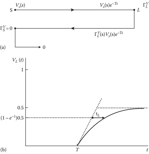
FIGURE 13.12
(a) Bounce diagram for Example 13.8, (b) sketch of load voltage for Example 13.8.

13.2.5Response to Nonlinear Terminations

As the clock speed of the computers increases into 10’s of GHz, the interconnect lengths of even centimeters will necessitate treating the interconnects as transmission lines (Chapter 4 of Reference 4). It is thus of interest to find a way to determine the evolution of the voltage or current pulse when the load is nonlinear, for example, a diode [3]. It is possible that both the source and the load have nonlinear V–I characteristics, for example, logic gates [4], where the interconnect has to be treated as a transmission line.

Example 13.9

Let the load in Figure 13.11 be a nonlinear resistor and the generator voltage be a step voltage as shown in Figure 13.13a.

Draw a Bergeron diagram to determine the evolution of the source end voltage V_S and the load end voltage V_L.

Solution

The diagram is shown in Figure 13.13b and is similar to Figure 13.3 except that the load line (L-line) is a curved line instead of a straight line.

The solid L-line is the V–I characteristic of the nonlinear resistor, and the solid line labeled as S-line is the V–I characteristic of the source terminal similar to the S-line in Figure 13.3. The dashed curves have slopes of plus or minus 45 degrees. The points S₁, S₂, etc. are the successive intersection points with the S-line and the 45-degree line. The points L₁, L₂, etc. are the intersection points of the L-line with the minus 45-degree line. The steady-state point (t approaches infinity) coincides with the intersection point of the S-line with the L-line, as expected.

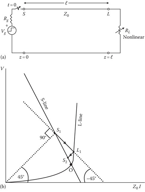
FIGURE 13.13
(a) Transmission line with a nonlinear resistive load. (b) Bergeron diagram for a nonlinear resistive load.

13.2.6Practical Applications of the Theory [1,2]

The simple theory presented above can be used to explain the principles of practical measuring and diagnostic devices to detect faults in inaccessible transmission lines like underground cables. The device is called time-domain reflectometer. Its principle is illustrated through Example 13.7. Some more examples are given as problems at the end of the chapter. More details can be obtained from [1,2].

13.3Transients on Lossy Transmission Lines

Equations 2.29 and 2.51 give the time-domain first-order coupled differential equations for the voltage V(z, t) and the current I(z, t) of a transmission line. These equations in s domain are given by

(13.33)

$- \frac{\partial V (z, s)}{\partial z} = (R^{'} + s L^{'}) I (z, s) - L^{'} I_{0} (z)$

(13.34)

$- \frac{\partial I (z, s)}{\partial z} = (G^{'} + s L^{'}) I (z, s) - C^{'} V_{0} (z),$

where I₀(z) is the initial current distribution and V₀(z) is the initial voltage distribution over the transmission line. Capital letters V and I are used for the time-domain functions as well as the s domain functions and where necessary, to avoid confusion, the argument of t or s is given in the parenthesis.

Assuming the line parameters are constant, we can obtain the second-order differential equations for the voltage:

(13.35)

$\begin{array}{l} \frac{d^{2} V (z, s)}{d z^{2}} - k^{2} (s) V (z, s) & = & L^{'} \frac{d}{d z} I_{0} (z) - C^{'} (R^{'} + s L^{'}) V_{0} (z) \\ k^{2} (s) & = & (R^{'} + s L^{'}) (G^{'} + s C^{'}) . \end{array}$

The solution of this second-order ordinary differential equation can now be obtained [5], the homogeneous part being

(13.36)

$V_{h} (z, s) = V_{0}^{+} (s) e^{- k (s) z} + V_{0}^{-} (s) e^{+ k (s) z}$

and the particular integral being

(13.37)

$V_{p} (z, s) = \frac{1}{2 k (s)} [e^{k (s) z} \int e^{- k (s) z} M_{v} (z) d z - e^{- k (s) z} \int e^{k (s) z} M_{v} (z) d z],$

where

(13.38)

$k (s) = \frac{1}{v_{0}} \sqrt{[{[(s + μ]}^{2} - ν^{2}]}$

(13.39)

$μ = \frac{1}{2} [\frac{R^{'}}{L^{'}} + \frac{G^{'}}{C^{'}}]$

(13.40)

$ν = \frac{1}{2} [\frac{R^{'}}{L^{'}} - \frac{G^{'}}{C^{'}}]$

(13.41)

$v_{0} = \sqrt{\frac{1}{L^{'} C^{'}}}$

and

(13.42)

$M_{v} (z) = L^{'} \frac{d}{d z} I_{0} (z) - C^{'} (R^{'} + s L^{'}) V_{0} (z) .$

In (13.38), (13.39), and (13.40), μ is not the permeability and ν is not the collision frequency. In this section, these symbols are used with a different meaning to be consistent with [6], whose approach is used to solve the problem by using the Laplace transform technique.

13.3.1Solution Using the Laplace Transform Technique

Let us assume that the line does not have any initial energy.

To obtain the main results of such a solution, let us assume that the line has zero initial energy, that is,

(13.43)

$V_{0} (z) = 0$

(13.44)

$I_{0} (z) = 0.$

Then the solution for V(z, s) is given by (13.36). The solution for I(z, s) is obtained by substituting (13.36) in (13.33) and is given by

(13.45)

$I (z, s) = I^{+} (z, s) + I^{-} (z, s)$

(13.46)

$I^{+} (z, s) = \frac{V^{+} (z, s)}{Z_{c} (s)}$

(13.47)

$I^{-} (z, s) = - \frac{V^{-} (z, s)}{Z_{c} (s)},$

where

(13.48)

$Z_{c} (s) = \sqrt{\frac{R^{'} + s L^{'}}{G^{'} + s C^{'}}}$

(13.49)

$Z_{c} (s) = Z_{0} \sqrt{\frac{s + (μ + ν)}{s + (μ - ν)}}$

(13.50)

$Z_{0} = \frac{L^{'}}{C^{'}} .$

13.3.1.1Loss-Free Line

If the line is loss free (R′ = 0, G′ = 0), we recover the equations we used for the ideal transmission line, since

(13.51)

$μ = 0, ν = 0,$

(13.52)

$k (s) = \frac{s}{v_{0}},$

(13.53)

$V (z, s) = V_{0}^{+} (s) e^{- s z / v_{0}} + V_{0}^{-} (s) e^{+ s z / v_{0}} .$

If $V_{0}^{+} (s)$ is the Laplace transform of $V_{0}^{+} (t)$ and $V_{0}^{-} (s)$ is the Laplace transform of $V_{0}^{-} (t)$ , the time-domain solution can be obtained as

(13.54)

$V (z, t) = V_{0}^{+} (t - \frac{z}{v_{0}}) + V_{0}^{-} (t + \frac{z}{v_{0}}) .$

The first term on the RHS of (13.54) is the positive-going wave and the second term is the negative-going wave.

13.3.1.2Distortionless Line

The second simple case occurs when

(13.55)

$\frac{R^{'}}{L^{'}} = \frac{G^{'}}{C^{'}} = μ and ν = 0,$

which was the condition for distortionless transmission line. In such a case

(13.56)

$k (s) = \frac{s + μ}{v_{0}} .$

The positive-going wave has the Laplace transform

$V_{0}^{+} (z, s) = V_{0}^{+} (s) e^{- (s + μ) z / v_{0}}$

(13.57)

$V_{0}^{+} (z, s) = V_{0}^{+} (s) e^{- μ z / v_{0}} e^{- s z / v_{0}}$

(13.58)

$V_{0}^{+} (z, t) = e^{- μ z / v_{0}} V_{0}^{+} (t - \frac{z}{v_{0}}) .$

As expected, the wave attenuates but travels without distortion.

13.3.1.3Lossy Line

When nu is not equal to zero, the signal gets distorted as it travels. Hence, ν is called the distortion constant. To study this quantitatively, we will take the Laplace inverse of exp[−k(s)z], that is, we take $V_{0}^{+} (s) = 1$ and $V_{0}^{+} (t) = δ (t)$ .

The Laplace inverse of exp[−k(s)z], where k(s) is given by (13.38), can be written as the sum of term1 and term2 [6]:

(13.59)

$t e r m 1 = e^{- μ z / ν_{0}} δ (t - \frac{z}{v_{0}})$

(13.60)

$t e r m 2 = ν^{2} a (z, t) u (t - \frac{z}{v_{0}}),$

where

(13.61)

$a (z, t) = (\frac{z}{v_{0}}) e^{- μ t} \frac{I_{1} [ν \sqrt{t^{2} - {(z / v_{0})}^{2}}]}{ν \sqrt{t^{2} - {(z / v_{0})}^{2}}} .$

In (13.60) u is the unit step function, and in (13.61) I is the modified Bessel function of the first kind. The term1 is the original impulse traveling along z with attenuation but no distortion and thus is the same solution as that of a distortionless line. The second term is the “wake” behind the distortionless wave. The wake is due to the dispersion and is sketched in Figure 13.14. The wake is zero for t < z/v₀. At t = z/v₀, it reaches a peak value:

(13.62)

$Peak value = \frac{ν^{2}}{2} \frac{z}{v_{0}} e^{- μ z / v_{0}} .$

For t > z/v₀, it decays with an asymptotic value given by Equation 4.44 of Reference [6] (Figure 13.14).

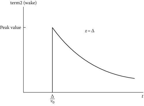
FIGURE 13.14
Sketch of the term2 given by (13.60), which is the wake behind the undistorted wave. The peak value is given by (13.62).

The solution for the current can be obtained on similar lines, and Reference [6] discusses this and other aspects of the solution of the lossy transmission line problem using the Laplace transform technique.

13.4Direct Solution in Time Domain: Klein–Gordon Equation

From Equations 2.49 and 2.51, when the transmission line parameters are constant, one can obtain easily the second-order PDE for the voltage V(z, t).

(13.63)

$\frac{\partial^{2} V}{\partial t^{2}} - v_{0}^{2} \frac{\partial^{2} V}{\partial z^{2}} + (\frac{R^{'}}{L^{'}} + \frac{G^{'}}{C^{'}}) \frac{\partial V}{\partial t} + (\frac{R^{'}}{L^{'}} \frac{G^{'}}{C^{'}}) V = 0.$

The solution in the time domain can be obtained by the following substitution:

(13.64)

$V (z, t) = e^{- μ t} U (z, t)$

in the time-domain equation for V(z, t). The function U(z, t) satisfies

(13.65)

$\frac{\partial^{2} U}{\partial t^{2}} - v_{0}^{2} \frac{\partial^{2} U}{\partial z^{2}} = ν^{2} U .$

Equation 13.33 is like the well-known Klein–Gordon equation of mathematical physics and is used to model a number of physical problems. Two simple examples are discussed below.

13.4.1Examples of Klein–Gordon Equation

A simple example is the model for the motion of a string of mass density ρ per meter length, under tension T, in an elastic medium like a thin rubber sheet of spring constant K. The PDE for the displacement ψ is given by [7]

(13.66)

$ρ \frac{\partial^{2} ψ}{\partial t^{2}} = T \frac{\partial^{2} ψ}{\partial z^{2}} - K ψ .$

This equation can be written as

(13.67a)

$\frac{\partial^{2} ψ}{\partial z^{2}} - \frac{1}{v_{s}^{2}} \frac{\partial^{2} ψ}{\partial t^{2}} = μ_{s}^{2} ψ,$

where

(13.67b)

$v_{s}^{2} = \frac{T}{ρ}$

(13.67c)

$μ_{s}^{2} = \frac{K}{T} .$

The dispersion equation for harmonic variations in space and time is given by

(13.68)

$ω^{2} = v_{s}^{2} k^{2} + μ_{s}^{2} v_{s}^{2} .$

Equation 13.68 is similar to the dispersion relation for a plasma medium or a waveguide with the feature of a cutoff frequency ω_c. In this case,

(13.69)

$ω_{c} = μ_{s} v_{s} .$

If the string is pinned down at z = 0 and z = L (Dirichlet BC), the solution can be easily found as

(13.70)

$ψ = ψ_{0} sin \frac{n π z}{L} e^{j ω_{n} t},$

where

(13.71)

$ω_{n}^{2} = v_{s}^{2} [{(n π / L)}^{2} + μ_{s}^{2}] .$

The allowed frequencies are larger because of the quantity $μ_{s}^{2}$ , which is proportional to the spring constant of the elastic medium [7].

A second example is the modeling of propagation of a uniform plane wave in an isotropic plasma medium of plasma frequency ω_p. Equation 9.10, Equation 9.11 and Equation 9.12 give the relevant equations for E, H, and J in the plasma medium. Eliminating H and J, we obtain

(13.72)

$\frac{\partial^{2} E}{\partial z^{2}} - \frac{1}{c^{2}} \frac{\partial^{2} E}{\partial t^{2}} = \frac{ω_{p}^{2}}{c^{2}} E .$

The dispersion relation and the cutoff frequency in this case are given by

(13.73)

$ω^{2} = k^{2} c^{2} + ω_{p}^{2}$

(13.74)

$ω_{c} = ω_{p} .$

Equation 13.72 can be transformed into the standard form of the KG equation

(13.75)

$\frac{\partial^{2} f}{\partial η^{2}} - \frac{\partial^{2} f}{\partial τ^{2}} = f$

by the following substitutions given in (13.76a), (13.76b), and (13.76c):

(13.76a)

$η = \frac{ω_{p} z}{c}$

(13.76b)

$τ = ω_{p} t$

(13.76c)

$E = E_{0} f .$

The nonsinusoidal time-domain exact solution of the KG equation (13.75) is given by Shvartsburg [8]:

(13.77)

$f = \sum_{q} E_{q} f_{q} (τ, η)$

(13.78)

$f_{q} (τ, η) = \frac{1}{2} [g_{q - 1} (τ, η) - g_{q + 1} (τ, η)]$

(13.79)

$g_{q} (τ, η) = {(\frac{τ - η}{τ + η})}^{q / 2} J_{q} (\sqrt{τ^{2} - η^{2}}),$

where J is the Bessel function of the first kind.

By changing η to jη and τ to jτ, Equation 13.75 can be transformed into

(13.80)

$\frac{\partial^{2} U}{\partial η^{2}} - \frac{\partial^{2} U}{\partial τ^{2}} = - U .$

Its solution is given by (13.77), (13.78) and (13.79) except that (13.79) changes to (13.81):

(13.81)

$g_{q} (τ, η) = {(\frac{τ - η}{τ + η})}^{q / 2} I_{q} (\sqrt{τ^{2} - η^{2}}), τ \geq η \geq 0.$

13.5Nonlinear Transmission Line Equations and KdV Equation

The circuit representation of a differential length of a nonlinear transmission line with dispersion that will be discussed in this section is shown in Figure 13.15.

FIGURE 13.15
Circuit representation of a differential length of a nonlinear transmission line.

Let us take a specific example where

(13.82)

$C_{N L}^{'} = C^{'} - C_{N}^{'} V .$

It can be shown that V(z, t) satisfies the nonlinear PDE [9]

(13.83)

$\frac{\partial^{2} V}{\partial z^{2}} - L^{'} C^{'} \frac{\partial^{2} V}{\partial t^{2}} + L^{'} C_{d}^{'} \frac{\partial^{4} V}{\partial z^{2} \partial t^{2}} + L^{'} C_{N}^{'} \frac{\partial^{2} (V^{2})}{\partial t^{2}} = 0.$

The first two terms on the LHS of (13.83) describe the wave propagation in an ideal transmission line. The third term arises because of the presence of the capacitor $C_{d}^{'}$ parallel to L′. Its effect can be studied by making $C_{N}^{'} = 0$ in (13.83). In such a case, the dispersion equation becomes

(13.84)

$\frac{ω}{k} = \frac{1}{\sqrt{L^{'} C_{d}^{'} k^{2} + L^{'} C^{'}}} .$

The sketch of the dispersion relation (13.84) is given in Figure 13.16.

FIGURE 13.16
Sketch of the dispersion relation given by Equation 13.84.

The third term causes the dispersion, while the fourth term provides the nonlinearity. In Section 9.10, it is mentioned that the balancing of the wave-steepening feature of nonlinearity can compensate the wave-flattening feature of the dispersion to preserve the signal shape as the wave propagates. This “soliton” aspect can be quantitatively studied by this model. In “TODA” model of the NLTL [10], the dispersion arises due to the use of a finite number of sections to represent the transmission line [10], where Δz = h, the length of each section. Such discretization provides numerical dispersion [11]. The study of the required parameter relationships between L′, C′, $C_{d}^{'}$ , and $C_{N}^{'}$ to obtain the needed balance between dispersion and nonlinearity to preserve the wave shape is facilitated by understanding the standard form of Korteweg-de-Vries (KdV) equation, whose solution is a “soliton.”

13.5.1Korteweg-de-Vries (KdV) Equation and Its Solution

The standard form of KdV equation and its solution are given below:

(13.85)

$\frac{\partial u}{\partial t} + 6 u \frac{\partial u}{\partial z} + \frac{\partial^{3} u}{\partial z^{3}} = 0$

(13.86)

$U (z, t) = A sec h^{2} [\sqrt{\frac{A}{2}} (z - 2 A t)] .$

By direct substitution of (13.86) in the third term on the LHS of (13.85), it can be shown [10] that

(13.87)

$U_{z z z} = - 2 A U_{z} - 6 U U_{z},$

where we follow the standard notation of the addition of a subscript to the symbol to denote its partial derivative with respect to the subscripted independent variable, that is,

(13.88)

$U_{z} = \frac{\partial U}{\partial z} .$

Equation 13.85 can now be written as

(13.89)

$U_{t} + 6 U U_{z} - 2 A U_{z} - 6 U U_{z} = 0.$

The nonlinear term 6UU_z, the second term in (13.89), cancels with the fourth term, which comes from the dispersion term U_zzz given in (13.87). We are now left with a linear equation

(13.90)

$U_{t} - 2 A U_{z} = 0,$

whose solution is given by (13.86). This can be shown by substitution of (13.86) in (13.90). A sketch of (13.86) is given in Figure 13.17. Its velocity is 2A, and its amplitude is A.

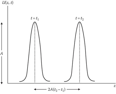
FIGURE 13.17
Sketch of a soliton given by Equation 13.86.

The solution (13.86) can also be obtained by solving (13.85) in the wave frame [9,10]

(13.91)

$ς = z - v_{s} t,$

where v_s is the velocity of the “solitary wave”; the velocity could be a function of the amplitude of the wave. Equation 13.85 transforms into

(13.92)

$- v_{s} u_{ς} + 6 u u_{ς} + u_{ς ς ς} = 0,$

where the subscript ζ is used as usual to denote the derivative with respect to ζ. Equation 13.92 is now an ordinary differential equation. Integrating it with respect to ζ, we get

(13.93)

$- v_{s} u + 3 u^{2} + u_{ς ς} = c_{1} .$

The pulse solution that satisfies zero values for u and its first- and second-order derivatives as the magnitude of ζ tends to infinity make c₁ = 0.

Multiplying (13.93) by u_ς, and recognizing the term u_ςςu_ς as $\frac{1}{2} \frac{d}{d ς} {(u_{ς})}^{2}$ , we get

(13.94)

$- v_{s} u u_{ς} + 3 u^{2} u_{ς} + \frac{1}{2} \frac{d}{d ς} {(u_{ς})}^{2} = 0.$

Integration of (13.94) with respect to ζ yields (13.95), where the integration constant c₂ is set to zero for the same reason that c₁ is set to zero.

(13.95)

$- v_{s} \frac{u^{2}}{2} + u^{3} + \frac{1}{2} {(u_{ς})}^{2} = 0.$

Solving (13.95) for u_ζ, we get (13.96)

(13.96)

$\frac{d u}{d ς} = {(v_{s} u^{2} - 2 u^{3})}^{1 / 2} .$

The solution of this first-order differential equation gives the relation of ζ with u. By transforming back to the lab frame in z , t, we get the solution given in (13.86).

13.5.2KdV Approximation of NLTL Equation

Equation 13.83 can be approximated by KdV equation for small amplitudes of the wave. Reductive perturbation method [9,10,12,13] is used to make this approximation. It begins by transforming from lab coordinates (z, t) to those of (S, T) in a reference frame that moves with a velocity v₀:

(13.97)

$v_{0} = \frac{1}{\sqrt{L^{'} C^{'}}}$

(13.98a)

$S = ε^{1 / 2} (z - v_{0} t)$

(13.98b)

$T = ε^{3 / 2} t .$

In the above, ε is called the “bookkeeping” parameter. The relations between the derivatives are

(13.99a)

$\frac{\partial}{\partial z} = ε^{1 / 2} \frac{\partial}{\partial S}$

(13.99b)

$\frac{\partial}{\partial t} = - ε^{1 / 2} v_{0} \frac{\partial}{\partial S} + ε^{3 / 2} v_{0} \frac{\partial}{\partial T} .$

The voltage V will be expressed in a perturbation series in powers of ε:

(13.100)

$V = ε u^{(1)} + ε^{2} u^{(2)} + \dots$

Substituting (13.97), (13.98), (13.99) and (13.100) in (13.83) and collecting terms of similar power in ε, one can obtain a series of equations. The lowest-order equation for u⁽¹⁾ is given by

(13.101)

$v_{0} \frac{\partial u^{(1)}}{\partial T} + \frac{C_{N}^{'}}{C^{'}} u^{(1)} \frac{\partial u^{(1)}}{\partial S} + \frac{C_{d}^{'}}{2 C^{'}} \frac{\partial^{3} u^{(1)}}{\partial S^{3}} = 0.$

By comparing (13.85), the standard form of KdV equation, with (13.101), the solution of (13.85) can be adapted to obtain the solution of (13.101). On transforming back to the lab coordinates z and t, we obtain [9]

(13.102)

$U (z, t) = U_{0} sec h^{2} [\sqrt{\frac{C_{N}^{'} U_{0}}{6 C_{d}^{'}}} (z - (1 + \frac{C_{N}^{'} U_{0}}{3 C^{'}}) \frac{t}{\sqrt{L^{'} C^{'}}})] .$

The velocity v_S of the wave solution in (13.102), called solitary wave, is given by [9]

(13.103)

$v_{S} = (1 + \frac{C_{N}^{'} U_{0}}{3 C^{'}}) \frac{1}{\sqrt{L^{'} C^{'}}} .$

The velocity increases with amplitude of the wave.

It can be noted that KdV equation (13.101) is a small-amplitude approximation of (13.83), since we approximated V by the first term u(1) in (13.100). For a comprehensive study of the theory, design, and applications of solitons, Reference [10] can be consulted. A few pointers from [10] that connect well with the material of this section are given below.

The “soliton” solution of the standard KdV equation (13.86) has a single parameter A, the amplitude of the soliton. The velocity of this pulse is amplitude dependent and is given by

(13.104)

$v_{S} = 2 A .$

A taller pulse travels faster than a shorter pulse. If A₁ and A₂ are the parameters of two solitons, and A₂ > A₁, the second (taller) pulse can collide with and overtake the first (shorter) pulse. While the two pulses interact nonlinearly during the collision, they can come out unaltered after the collision. This characteristic distinguishes a soliton [14] from other solitary wave solutions with hyperbolic secant profiles. Two such examples of differential equations are given in [10].

13.6Charged Particle Dynamics [15,16]

13.6.1Introduction

Electromagnetic force on a charged particle of charge q in electric and magnetic fields is given by (1.6) and is repeated here as (13.105)

(13.105)

$F = q (E + ν \times B) .$

One can derive from (13.105) the concepts of and equations relating force density f, Maxwell’s stress tensor $\bar{T}$ , and electromagnetic momentum g in a volume V bounded by a surface s due to charge density ρ and current density J.

This aspect is discussed in Appendix 13A rather than here to maintain the narrative of the charged particle dynamics. The Newton’s second law (see Appendix 13B, for discussion of the validity of Newton’s third law to forces on charged particles) gives

(13.106)

$F = m a,$

where

(13.107)

$a = \frac{d v}{d t} = \frac{d^{2} r}{d t^{2}} .$

In (13.107) r is the position vector of the point where the charged particle is located. Thus, we will write (13.108) as the starting equation to study the charged particle dynamics.

(13.108)

$m \frac{d v}{d t} = m \frac{d^{2} r}{d t^{2}} = q (E + ν \times B) .$

We used (13.108) with appropriate approximations to model dielectrics, conductors, and plasmas in Chapters 8, 9, and 11. In Section 13.8, we will use an appropriate approximation of (13.108) to model magnetohydrodynamics (MHD), which is a study of moving liquid conductors. However, in this section, we study the pertinent aspects of the dynamics of a charged particle. First we study in the next section the kinematics, that is, the expressions for the velocity v and acceleration a given the trajectory, thus separating this aspect from the aspect of specific forces that produced this trajectory.

13.6.2Kinematics

Figure 13.18 gives a sketch of a general curve and a typical point P on the curve with reference to the origin O of a coordinate system.

FIGURE 13.18
Sketch showing the position vector r, velocity v, and acceleration a of a particle moving along a trajectory.

In Cartesian coordinate system, the position vector r, the directed line segment OP, shown in the figure is given by

(13.109)

$r (t) = \overset{⌢}{x} x (t) + \overset{⌢}{y} y (t) + \overset{⌢}{z} z (t) .$

The time derivatives d/dt (sometimes denoted by a dot on the top) of the unit vectors x, y, and z are zero since they are constant unit vectors. Thus,

(13.110)

$v (t) = \frac{d}{d t} r (t) = \dot{r} (t) = \overset{⌢}{x} \dot{x} (t) + \overset{⌢}{y} \dot{y} (t) + \overset{⌢}{z} \dot{z} (t)$

(13.111)

$a (t) = \dot{v} (t) = \frac{d^{2}}{d t^{2}} r (t) = \ddot{r} (t) = \overset{⌢}{x} \ddot{x} (t) + \overset{⌢}{y} \ddot{y} (t) + \overset{⌢}{z} \ddot{z} (t) .$

In cylindrical coordinates, the trajectory will be given in terms of ρ(t), ϕ(t), z(t) and the unit vectors $\overset{⌢}{ρ}$ , $\overset{⌢}{ϕ}$ , $\overset{⌢}{z}$ . Note that the unit vectors in this case are not constant and depend on the azimuthal coordinate ϕ. See Appendix 1A. The position vector is given by

(13.112)

$r = \overset{⌢}{ρ} (ϕ) ρ + \overset{⌢}{z} z,$

where

(13.113)

$\overset{⌢}{ρ} (ϕ) = \overset{⌢}{x} cos ϕ (t) + \overset{⌢}{y} sin ϕ (t)$

(13.114)

$\overset{⌢}{ϕ} (ϕ) = - \overset{⌢}{x} sin ϕ (t) + \overset{⌢}{y} cos ϕ (t) .$

From (13.113),

$\begin{array}{c} \frac{d}{d t} \overset{⌢}{ρ} (ϕ) & = & \overset{⌢}{x} \frac{d}{d t} cos ϕ (t) + \overset{⌢}{y} \frac{d}{d t} sin ϕ (t) \\ = & \overset{⌢}{x} \frac{d}{d ϕ} cos ϕ \frac{d ϕ}{d t} + \overset{⌢}{y} \frac{d}{d ϕ} sin ϕ \frac{d ϕ}{d t} \\ = & - \overset{⌢}{x} sin ϕ \frac{d ϕ}{d t} + \overset{⌢}{y} cos ϕ \frac{d ϕ}{d t} . \end{array}$

From (13.114),

(13.115)

$\frac{d}{d t} \overset{⌢}{ρ} (ϕ) = \overset{⌢}{ϕ} \frac{d ϕ}{d t} .$

Proceeding on similar lines, we can obtain Equation 13.116, Equation 13.117, Equation 13.118, Equation 13.119 and Equation 13.120:

(13.116)

$\frac{d}{d t} \overset{⌢}{ϕ} (ϕ) = - \overset{⌢}{ρ} \frac{d ϕ}{d t}$

(13.117)

$\frac{d^{2}}{d t^{2}} \overset{⌢}{ρ} (ϕ) = - \overset{⌢}{ρ} {[\dot{ϕ}]}^{2} + \overset{⌢}{ϕ} \frac{d^{2} ϕ}{d t^{2}}$

(13.118)

$\frac{d^{2}}{d t^{2}} \overset{⌢}{ϕ} (ϕ) = - \overset{⌢}{ρ} \frac{d^{2} ϕ}{d t^{2}} - \overset{⌢}{ϕ} {[\dot{ϕ}]}^{2}$

(13.119)

$v (t) = \frac{d^{2}}{d t^{2}} r (t) = \dot{r} (t) = \overset{⌢}{ρ} \dot{ρ} + \overset{⌢}{ϕ} ρ \dot{ϕ} + \overset{⌢}{z} \dot{z}$

(13.120)

$a (t) = \dot{v} (t) = \frac{d^{2}}{d t^{2}} r (t) = \ddot{r} (t) = \overset{⌢}{ρ} [\ddot{ρ} - ρ {(\dot{ϕ})}^{2}] + \overset{⌢}{ϕ} [ρ \ddot{ϕ} + 2 \dot{ρ} \dot{ϕ}] + \overset{⌢}{z} \dot{z} .$

The second term in the multiplier of the unit vector $\overset{⌢}{ρ}$ in (13.120) gives the so-called centripetal acceleration a_cp:

(13.121)

$a_{c p} = \overset{⌢}{ρ} [- ρ {(\dot{ϕ})}^{2}],$

which, because of the negative sign, is directed toward the axis of the cylinder.

The second term in the multiplier of the unit vector $\overset{⌢}{ϕ}$ is called Coriolis acceleration a_CL:

(13.122)

$a_{C L} = \overset{⌢}{ϕ} [2 \dot{ρ} \dot{ϕ}] .$

For a circular motion in the x–y plane (ρ = ρ₀, z = 0), the expressions given in (13.112), (13.119), and (13.120) for the position vector, velocity, and acceleration, respectively, can be further simplified and are given by (13.123), (13.124) and (13.125):

(13.123)

$r = \overset{⌢}{ρ} (ϕ) ρ_{0}$

(13.124)

$v (t) = \overset{⌢}{ϕ} ρ_{0} ω$

(13.125)

$a (t) = \overset{⌢}{ρ} [- ρ_{0} {(ω)}^{2}] + \overset{⌢}{ϕ} ρ_{0} α,$

where $ω = \dot{ϕ}$ is the instantaneous angular velocity and $α = \ddot{ϕ}$ is the instantaneous angular acceleration.

13.6.3Conservation of Particle Energy due to Stationary Electric and Magnetic Fields

Let us start with the assumption that the electric and magnetic fields are not varying in time. By taking the dot product of (13.108) with v, and using E = − ∇Φ, we obtain the following energy conservation law:

(13.126)

$\frac{d}{d t} (\frac{1}{2} m v^{2} + q Φ) = 0.$

The first term in the parenthesis is the kinetic energy and the second term is the potential energy of the particle. The total energy of the particle is conserved due to its motion, in electric and magnetic fields not varying in time.

13.6.4Constant Electric and Magnetic Fields

Let us consider the case of constant electric and magnetic fields. Without loss of generality, we can assume the magnetic field is in the z-direction. Then we can write the vector differential equation (13.108) as three scalar differential equations:

(13.127)

${\dot{v}}_{x} = \frac{q}{m} (E_{y} + B v_{y})$

(13.128)

${\dot{v}}_{y} = \frac{q}{m} (E_{y} - B v_{x})$

(13.129)

${\dot{v}}_{z} = \frac{q}{m} E_{z} .$

Equations 13.127 and 13.128 are coupled and by differentiating (13.127) and substituting for ${\dot{v}}_{y}$ , we obtain

(13.130)

${\ddot{v}}_{x} + ω_{b}^{2} v_{x} = ω_{b}^{2} \frac{E_{y}}{B} .$

Equation 13.130 is a second-order differential equation and its solution is easily obtained:

(13.131)

$v_{x} = A sin (ω_{b} t - δ) + \frac{E_{y}}{B} .$

The first term on the RHS is the homogeneous part of the solution with two undetermined constants A and δ. The second term is the particular integral. After obtaining ${\dot{v}}_{x}$ from (13.131) and substituting it in (13.127), one can obtain v_y:

(13.132)

$v_{y} = A cos (ω_{b} t - δ) - \frac{E_{x}}{B} .$

The particular integrals in (13.131) and (13.132) can be written in a more general vectorial form

(13.133)

$v_{D E} = \frac{E \times B}{B^{2}},$

where v_DE is called the drift velocity due to the electric field, which is independent of the mass and charge of the particle. Both the electrons and positive ions drift along together. The homogeneous part of the solutions given in (13.131) and (13.132) are oscillations at the gyrofrequency ω_b. The drift velocity is zero if E and B are in the same direction or if E is zero. Let us consider in more detail the motion of the particle for the second case of E = 0.

13.6.4.1Special Case of E = 0

Since the potential energy is zero, from (13.126), the kinetic energy of the particle is a constant of motion in the x–y plane (plane perpendicular to the B field). The magnitude of the velocity v is a constant of motion.

Let us take a concrete case by specifying the following initial conditions v_x(0) = 0 and v_y(0) = v₀. Since E = 0, the harmonic solution for v_x and v_y will be chosen from sin or cos type from the template like (3.15) that satisfies the given initial conditions:

(13.134)

$v_{x} (t) = v_{0} sin ω_{b} t$

(13.135)

$v_{y} (t) = v_{0} cos ω_{b} t .$

The expressions for x and y coordinates of the particle can be obtained by integrating (13.134) and (13.135) and will be again trigonometric type multiplied by of v₀/ω_b. If the initial conditions are x(0) = − ρ₀ and y(0) = 0, the trajectory of the charged particle in the x–y plane is given by

(13.136)

$x (t) = - ρ_{0} cos ω_{b} t$

(13.137)

$y (t) = ρ_{0} sin ω_{b} t,$

where

(13.138)

$ρ_{0} = \frac{v_{0}}{ω_{b}} .$

This trajectory is a circle of radius ρ₀ centered at the origin in the transverse plane as sketched in Figure 13.19.

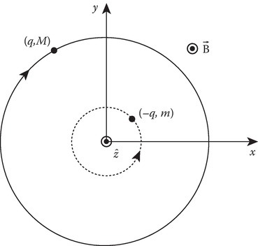
FIGURE 13.19
Sketch of circular trajectories of charged particles in the plane perpendicular to the static magnetic field. Note that the radius and the sense of rotation for an electron is different from those for a positive ion like a proton.

For an ion of positive charge q and mass M, the particle rotates clockwise as shown by the solid line. For an electron of negative charge (–q) and mass m, ω_b is negative and larger in magnitude than for the case of ion, and the electron rotates counterclockwise as sketched in the figure with a dotted line. The radius of the circle ρ₀ is called radius of gyration or cyclotron radius of the particle. This circular motion is already described from the kinematic viewpoint in Equations 13.123 and 13.124 when we identify the angular velocity ω with the particle gyrofrequency ω_b.

Equation 13.129 for the case of E = 0 has a simple solution, and for the assumed initial conditions of v_z(0) = v₁ and z(0) = 0,

(13.139)

$v_{z} (t) = v_{1}$

(13.140)

$z (t) = v_{1} t .$

Thus, the particle trajectory is helical in the three-dimensional space.

Let us state in words the results we obtained so far in this section. The combination of the parallel component of E and the B field produces only uniform motion of the charged particle. The B field has no effect. The combination of the perpendicular component of E and the B field produces a moving circular orbit whose center, called the guiding center, moves with a drift velocity given by (13.133). Note that the drift takes place in the transverse plan normal to the perpendicular component of the E field. Magnitude of the drift velocity does not depend on the charge or mass of the particle. It depends on the ratio of the magnitude of the transverse component of the electric field to that of the B field. See Figure 13.20.

FIGURE 13.20
Sketches of the trajectories of positive and negative charges. The B field is in the z-direction, and the perpendicular component of the electric field is in the y-direction.

13.6.5Constant Gravitational Field and Magnetic Field

In this section, we replace the electric field with the gravitational field and consider the solution of the equation

(13.141)

$m \frac{d v}{d t} = m \frac{d^{2} r}{d t^{2}} = m g + q (v \times b),$

where g is the acceleration due to gravity. Comparing (13.108) with (13.141), we note that the drift velocity in this case will be given by

(13.142)

$v_{D g} = \frac{m}{q} \frac{g \times B}{B^{2}} .$

In this case the drift velocity does depend on the mass and the algebraic value of the charge. The electrons and ions have drift in opposite directions. We can generalize the formula for the drift velocity when we replace the electric force E in (13.133) by a general external force F:

(13.143)

$v_{D F} = \frac{1}{q} \frac{F \times B}{B^{2}} .$

13.6.6Drift Velocity in Nonuniform B Field

In this section, we will discuss the motion of a charged particle in a slightly nonuniform but static B field. As a specific example, let us calculate the drift velocity, the velocity of the guiding center of the trajectory, in a z-directed B field with a small gradient in the x-direction. If the imposed B field is in free space, it has to satisfy the following two equations:

(13.144)

$\nabla \cdot B = 0$

(13.145)

$\nabla \times B = 0.$

Tannenbaum [15] considers the following expression for the B field, which satisfies (13.144) and (13.145):

(13.146)

$B = B_{0} [\overset{⌢}{x} α z + \overset{⌢}{z} (1 + α x)] .$

If the parameter α is zero, we have the uniform B case considered in the previous section. If αz and αx are small compared to one, we have slightly nonuniform and nearly uniform static magnetic field. Since

(13.147)

$\nabla B_{z} = \overset{⌢}{x} α B_{0}, (113)$

the second term in the z-component of the B field in (13.146) will be called the “gradient” term. The first term on the RHS of (13.146), which is the x component of B, will be called the “curvature” term. A sketch of the B field line near the origin that goes through the origin of the x–z plane is shown in Figure 13.21. Its equation is given by [15]

(13.148)

${(x - \frac{1}{α})}^{2} + z^{2} = \frac{1}{α^{2}} .$

The solution for the velocities is obtained using a perturbation technique for the case αx ≪ 1 and αz ≪ 1. The end result for the drift velocity is given by

(13.149)

$v_{D} = \overset{⌢}{y} \frac{α}{ω_{b}} (\frac{1}{2} v_{0}^{2} + v_{1}^{2}) .$

The term ω_b in (13.149) shows that the drift velocity for a positive charge is in opposite direction to that of the negative charge.

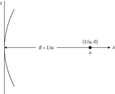
FIGURE 13.21
Curved B field line passing through the origin. See Equation 13.148.

The generalization of (13.149) is obtained by noting that the factor $\hat{y} α$ in (13.149) can be written as

(13.150)

$\overset{⌢}{y} α = \frac{B_{0} \times \nabla B_{z}}{B_{0}^{2}} = \frac{R \times B_{0}}{R^{2} B_{0}},$

where the radius of curvature

(13.151)

$R = \frac{- \overset{⌢}{x}}{α},$

as shown in Figure 13.21. Equation 13.149 can now be written as [15]

(13.152)

$v_{D} = \frac{v_{0}^{2}}{2 ω_{b}} \frac{B_{0} \times \nabla B_{z}}{B_{0}^{2}} + \frac{v_{1}^{2}}{ω_{b}} \frac{R \times B_{0}}{R^{2} B_{0}} .$

The first term on the RHS of (13.152) is called Grad-B drift, when Grad-B is perpendicular to B. The second term is called curvature drift.

13.6.7Time-Varying Fields and Adiabatic Invariants

We showed earlier that the charged particle trajectory in a uniform B field is a circle of radius ρ₀, relabeled here as ρ_L for Larmor radius. The circular motion is periodic, with a period

(13.153)

$t_{B} = \frac{1}{f_{B}} = \frac{2 π}{ω_{B}} = \frac{2 π m}{|q| B} .$

The velocity of the particle will be denoted by v_⊥ and its kinetic energy by w_⊥:

(13.154)

$w_{⊥} = \frac{1}{2} m v_{⊥}^{2},$

where

(13.155)

$w_{⊥} = ω_{B} ρ_{L} .$

If B is uniform, w_⊥ is a constant of motion.

If B is slowly varying, the trajectory is not a closed circle; nevertheless one can still approximate it as a closed path. In such an approximation, we can use the concept of action integral defined in (13.183) and use the property of constant of motion identifying the generalized momentum p with the transverse component of the particle momentum and the generalized differential coordinate dq with the differential length element of the closed path. The slowness can be defined by

(13.156)

$Δ B = \frac{\partial B}{\partial t} t_{B} \propto ω B t_{B} \propto \frac{t_{B}}{t_{s}} B = \frac{ω}{ω_{b}} B,$

where ΔB is the change in B in one gyration. In the above equation, t_s is the characteristic time scale of the B field variation. The slow change is called “adiabatic” and the conserved variables are called “adiabatic invariants” denoted by the symbol J, not to be confused with the volume current density. These are stated in various ways [17]:

(13.157)

$J_{1} \propto B ρ_{L}^{2}$

(13.158)

$J_{2} \propto \frac{p_{⊥}^{2}}{B}$

(13.159)

$J_{3} \propto μ_{m} .$

In the above, the symbol p_⊥ is the linear momentum of the charged particle in circular motion and μ_m is the magnetic dipole moment (abbreviated as magnetic moment) defined as p_m in (8.144). For the relativistic velocities (Chapter 14), the RHS of (13.159) will have a multiplier of the Lorentz factor γ.

We shall next consider the evaluation of (8.114) for the magnetic moment for a particle of positive charge q with a circular trajectory, shown in Figure 13.19, in a constant B field. Since its trajectory is clockwise, the direction of the vector area S of the circle is in opposite direction of the B field. The current I is the charge q multiplied by f_B.

(13.160)

$μ_{m} I S = q (\frac{ω_{b}}{2 π}) π ρ_{L}^{2} (\overset{⌢}{B}) = - \frac{1}{2} \frac{m v_{⊥}^{2}}{B} \overset{⌢}{B}$

(13.161)

$μ_{m} = \frac{w_{⊥}}{B} .$

If we use for the generalized coordinate p the angular momentum mv_⊥ρ_L and for q the coordinate ϕ in (13.183), we obtain

(13.162)

$J_{3} = \oint p d q = \oint m v_{⊥} ρ_{L} d ϕ = \frac{2 π m v_{⊥}^{2}}{ω_{b}} = 4 π \frac{m}{q} μ_{m} .$

Thus, μ_m is a constant of motion. However, for relativistic velocities it is γμ_m that is a constant of motion. The magnetic flux Φ_m through a Larmor orbit is

(13.163)

$Φ_{m} = π ρ_{L}^{2} B = \frac{2 π m}{q^{2}} μ_{m} .$

It is a constant of motion as long as μ_m is a constant of motion. Equation 13.157 is thus proved. Consequently, as the B field changes, the Larmor radius of the particle orbit changes suitably to preserve the magnetic flux through the area of the orbit.

It should be noted that the B field here is an imposed one and there is no imposed electric field. However, the changing magnetic field, according to Faraday’s law (1.1), gives rise to an induced electric field, denoted by E_⊥. Consequently the equation of motion

(13.164)

$\frac{d}{d t} (\frac{1}{2} m v_{⊥}^{2}) = q v_{⊥} \cdot E_{⊥} .$

It can be shown [18] that the change of the kinetic energy per gyration, Δw_⊥, is given by

(13.165)

$Δ w_{⊥} = Δ B \frac{w_{⊥}}{B} + O (ε^{2}) w_{⊥} .$

13.6.8Lagrange and Hamiltonian Formulations of Equations of Motion

The equations of motion can be obtained by more advanced formulations than Newtonian mechanics, which are essentially based on F = ma. Lagrange formulation is based on D’Alembert’s principle and the principle of virtual work [19]. The relevant equation in generalized coordinates is

(13.166)

$\frac{d}{d t} (\frac{\partial T}{\partial {\dot{q}}_{j}}) - (\frac{\partial T}{\partial q_{j}}) = Q_{j}$

(13.167)

$T = \sum \frac{1}{2} m_{i} v_{i}^{2} .$

In the above equation, q_j is the generalized coordinate, which need not have the dimension of length. Q_j is the component of the generalized force. It can be shown that (13.166) reduces to Newton’s second law F = ma = dp/dt; if q is the position coordinate, Q is the corresponding component of the force F, and p = mv is the momentum.

If Q_j can be written in terms of a generalized potential U, that is,

(13.168)

$Q_{j} = \frac{d}{d t} (\frac{\partial U}{\partial {\dot{q}}_{j}}) - (\frac{\partial U}{\partial q_{j}}),$

then (13.166) can be written as

(13.169)

$\frac{d}{d t} (\frac{\partial L}{\partial {\dot{q}}_{j}}) - (\frac{\partial L}{\partial q_{j}}) = 0.$

Here the Lagrangian L is given by

(13.170)

$L = T - U . (136)$

We shall next obtain the Lagrangian for describing the motion of a charged particle in an electromagnetic field. The electric field E in terms of the electric scalar potential Φ and the vector magnetic potential A is given by (1.8) and repeated here for convenience:

(13.171)

$E = - \nabla ϕ - \frac{\partial A}{\partial t} .$

Substituting (13.171) and (1.7) in the force equation (1.6), we get

(13.172)

$F = q (- \nabla Φ - \frac{\partial A}{\partial t} + v \times \nabla \times A) .$

Equation 13.172 can be written in a more convenient form. Its x-component

(13.173)

$F_{x} = - \frac{\partial U}{\partial x} + \frac{d}{d t} (\frac{\partial U}{\partial v_{x}}),$

where

(13.174)

$U = q Φ - q A \cdot v .$

From (13.168), (13.173), and (13.174), it is obvious that U is a generalized potential. If we consider the case of motion of a charged particle in an electrostatic field, then

(13.175)

$U = q Φ, (electrostatic case),$

which is the potential energy, and the Lagrangian is equal to the kinetic energy minus the potential energy. The Lagrangian for the electromagnetic case is given by

(13.176)

$L = \frac{1}{2} m v^{2} + q A \cdot v - q Φ .$

In the relativistic case, discussed in Chapter 14, since mass varies with velocity, L_rel is given by [18]

(13.177)

$L_{r e l} = - m_{0} (1 - \frac{v^{2}}{c^{2}}) + q A \cdot v - q Φ,$

where m₀ is the rest mass.

13.6.8.1Hamiltonian Formulation

In the Hamiltonian formulation of equations of motion, the independent generalized coordinates are (q, p, t) instead of $(q, \dot{q}, t)$ , where p’s are called generalized momenta, defined by

(13.178)

$p_{i} = \frac{\partial L (q_{j}, {\dot{q}}_{j}, t)}{\partial {\dot{q}}_{i}} .$

It can be shown [19], using Legendre transformation, that the following first-order differential equations describe the motion:

(13.179)

$\frac{d q_{i}}{d t} = \frac{\partial H}{\partial p_{i}}$

(13.180)

$\frac{d p_{i}}{d t} = - \frac{\partial H}{\partial q_{i}},$

where the Hamiltonian ℋ is related to the Lagrangian L by

(13.181)

$H (p, q, t) = \sum_{i} {\dot{q}}_{i} p_{i} - L (q, \dot{q}, t)$

(13.182)

$\frac{\partial H}{\partial t} = - \frac{\partial L}{\partial t} .$

Equations 13.179 and 13.180 are called canonical equations of Hamilton. The canonical variables p and q are independent variables. For each coordinate q, which is periodic, the action integral J is

(13.183)

$J = \oint p d q$

and is invariant.

We can further show that if L, and hence $H$ , is not an explicit function of t,

(13.184)

$\frac{d H}{d t} = \frac{\partial H}{\partial t} .$

For a charged particle,

(13.185)

$H = \frac{1}{2 m} {|(p - q A)|}^{2} + q Φ .$

In the above equation, p is the mechanical momentum.

For an electrostatic field, A is zero, and the Hamiltonian is kinetic energy (K.E.) plus potential energy (P.E.):

(13.186)

$H = \frac{p^{2}}{2 m} + q Φ = \frac{1}{2} m v^{2} + q Φ$

(13.187)

$H = K . E . + P . E . (electrostatic field) .$

For the same case, the Lagrangian L

(13.188)

$L = K . E . - P . E . (electrostatic case) .$

For the relativistic case,

(13.189)

$H_{r e l} = {[m_{0}^{2} c^{4} + c^{2} {|(p - q A)|}^{2}]}^{1 / 2} + q Φ .$

An example [20] of using the generalized coordinates and Hamiltonian formulation is given below.

13.6.8.2Photon Ray Theory

Photon ray theory is based on the geometrical optics concepts of propagation of electromagnetic wave packets in a medium. We will start with an x-polarized uniform plane wave propagating in a uniform medium in z-direction. Its electric field is given by

(13.190)

$E_{x} (z, t) = E_{0} (z, t) e^{j (ω t - k z)} .$

If the propagation is taking place in a slowly varying medium, we can modify (13.190) by

(13.191)

$E_{x} (z, t) = E_{0} (z, t) e^{j ψ (z, t)} .$

Where ψ is the wave phase and E₀ is a slowly varying amplitude. We can now define instantaneous values of frequency ω and wave number k by

(13.192a)

$k = - \frac{\partial ψ}{\partial z}$

(13.192b)

$ω = \frac{\partial ψ}{\partial t} .$

The local dispersion relation

(13.193)

$ω = ω (k, z, t)$

can be established when the properties of the medium (the refractive index n for a dielectric and the plasma frequency ω_p for a plasma medium) are known.

(13.194)

$\frac{\partial k}{\partial t} = - \frac{\partial}{\partial t} \frac{\partial ψ}{\partial z} = - \frac{d}{d z} \frac{\partial ψ}{\partial t} = - \frac{d ω}{d z} = - [\frac{\partial ω}{\partial z} + \frac{\partial ω}{\partial k} \frac{\partial k}{\partial z}]$

(13.195)

$\frac{\partial k}{\partial t} = - [\frac{\partial ω}{\partial z} + v_{g} \frac{\partial k}{\partial z}],$

where we define v_g as the group velocity:

(13.196)

$v_{g} = \frac{\partial ω}{\partial k} .$

The last term on the RHS of (13.194) arises since ω is also a function of k. Equation 13.193 can also be written as

(13.197)

$\frac{\partial k}{\partial t} + v_{g} \frac{\partial k}{\partial z} = - \frac{\partial ω}{\partial z} .$

If v_g is also the group velocity of the propagating wave packet, the LHS of (13.197) can be written as the total derivative dk/dt. Thus, we get the Equation 13.198 akin to the second of the Hamiltonian pair (13.180):

(13.198)

$\frac{d k}{d t} = - \frac{\partial ω}{\partial z} .$

The group velocity v_g can also be written in terms of the position of the centroid of the wave packet, that is, dr/dt. In our example of the one-dimensional wave, it is given by dz/dt. Thus, we get the first of the pair of the Hamiltonian canonical equations, like (13.179), by equating v_g obtained in two ways:

(13.199)

$\frac{d z}{d t} = \frac{\partial ω}{\partial k} .$

In this example, the generalized coordinates are z and k, and the Hamiltonian is ω(k, z, t). The energy E of a photon is hf = hω/2π = ℏω and the momentum of the photon is ℏk.

From (13.181) and the Hamiltonian analogy, the Lagrangian L for a photon can be written as

(13.200)

$L (z, v_{g}, t) = v_{g} k - ω (z, k, t) .$

The Lagrange equation for the photon is given by

(13.201)

$\frac{d}{d t} (\frac{\partial L}{\partial v_{g}}) - (\frac{\partial L}{\partial z}) = 0.$

Note from (13.200)

(13.202a)

$\frac{\partial L}{\partial v_{g}} = k$

(13.202b)

$\frac{\partial L}{\partial z} = - \frac{\partial ω}{\partial z} .$

Thus, (13.201) is the same as (13.198), repeated here as (13.203):

(13.203)

$\frac{d k}{d t} = - \frac{\partial ω}{\partial z} .$

If k is like momentum and ω is like energy, Equation 13.203 is like Newton’s law of motion. Also note that (13.203) is akin to the second of the Hamiltonian canonical pair for the photon given by (13.180).

Photon in vacuum has zero mass and zero charge. However, one can consider it having an effective mass m_eff and equivalent charge q_ph in a medium [20]. For example, Mendonca [20] arrives at the following values for these in an isotropic cold electron plasma of plasma frequency ω_p:

(13.204)

$m_{e f f} = \frac{ω_{p} ℏ}{c^{2}}$

(13.205)

$q_{p h} = - ℏ \frac{e k_{p}^{2}}{m_{e f f} ω_{0}}$

(13.206)

$k_{p} = \frac{ω_{p}}{v_{g}},$

where m_eff and e are the mass and absolute value of the charge, respectively, of an electron. ω₀ is the central frequency and v_g is the group velocity of the wave packet. These concepts help explain [20] the “ponderomotive force,” photon-beam plasma instabilities, etc. Ponderomotive force is due to the radiation pressure of the photon gas exerted on the electrons of the plasma.

Equations 13.204 and 13.205 give the effective mass and the equivalent charge of a “dressed” particle in contrast to the characterization of a photon in vacuum as a bare particle [20] of zero mass and zero charge.

13.6.8.3Space and Time Refraction Explained through Photon Theory [20]

We can use the above mentioned photon theory based on the Hamiltonian to explain the constancy of the frequency ω at a spatial discontinuity and the constancy of the wave number k at a temporal discontinuity of a medium. A temporal discontinuity consequently causes a change in the frequency. This aspect will be pursued more extensively in Section 13.9 based on Maxwell’s equations and full wave theory.

We generalize the direction of wave propagation by writing Equation 13.191, Equation 13.192a and Equation 13.192b in a generalized form:

(13.207)

$E_{x} (z, t) = E_{0} (z, t) e^{j ψ (r, t)}$

(13.208a)

$k = - \nabla ψ (32 a)$

(13.208b)

$ω = \frac{\partial ψ}{\partial t} .$

The Hamiltonian pair is given by

(13.209)

$\frac{d k}{d t} = - \nabla ω$

(13.210)

$\frac{d r}{d t} = \nabla_{k} ω .$

As long as ω is not an explicit function of time, we also have

(13.211)

$\frac{d ω}{d t} = \frac{\partial ω}{\partial t} . (35)$

Consider a dielectric medium [20] with

(13.212)

$ω = \frac{k c}{n} .$

From (13.210),

$\frac{d r}{d t} = \nabla_{k} ω = \frac{\partial}{\partial k} \frac{k c}{n} \overset{⌢}{k} = \frac{c}{n} \overset{⌢}{k} = \frac{c k}{n} \frac{k}{k^{2}} = \frac{ω k}{k^{2}}$

(13.213)

$\frac{d r}{d t} = \frac{ω k}{k^{2}} .$

From (13.209),

(13.214)

$\begin{array}{l} \frac{d k}{d t} = - \nabla ω = \frac{\partial}{\partial r} \frac{k c}{n} \overset{⌢}{r} = \frac{k c}{n^{2}} \frac{\partial n}{\partial r} \overset{⌢}{r} = \frac{ω}{n} \frac{\partial n}{\partial r} \overset{⌢}{r} = ω \nabla ln (n) \\ \frac{d k}{d t} = ω \nabla ln (n) . \end{array}$

From (13.211),

(13.215)

$\begin{array}{l} \frac{d ω}{d t} = \frac{\partial ω}{\partial t} = \frac{\partial}{\partial t} (\frac{k c}{n}) = - \frac{k c}{n^{2}} \frac{\partial n}{\partial t} = - \frac{ω}{n} \frac{\partial n}{\partial t} = - ω \frac{\partial}{\partial t} [ln (n)] \\ \frac{d ω}{d t} = - ω \frac{\partial}{\partial t} [ln (n)] . \end{array}$

Let us now consider two separate cases of n being a function of only one independent variable.

Case 1 Let

(13.216)

$n (r, t) = n (z),$

where n(z) is a step function shown in Figure 13.22.

From (13.215),

(13.217a)

$\frac{d ω}{d t} = 0$

(13.217b)

$ω = constant .$

Thus, we get the well-known result that the frequency of the incident, reflected, and the transmitted waves is the same, as stated in (2.90). From (13.214) and (13.216), since n is a function of z, the x-component of k = k_x satisfies

(13.218a)

$\frac{d k_{x}}{d t} = 0$

(13.218b)

$k_{x} = constant .$

The x-component of k is the same for the incident, reflected, and the transmitted waves, from which we get the well-known Snell’s law, normally stated as in (2.91) and shown in Figure 13.22.

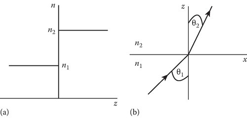
FIGURE 13.22
Refraction at a spatial discontinuity: (a) spatial step profile of the refractive index and (b) refraction at the spatial boundary.

Case 2 Let

(13.219)

$n (r, t) = n (t)$

where n(t) is a step function and the wave is propagating in the z-direction, that is, $k = \overset{⌢}{z} k$ .

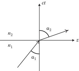
FIGURE 13.23
Refraction of a photon at a temporal discontinuity.

Since, in this case, n is not a function of z, from (13.214)

(13.220a)

$\frac{d k}{d t} = 0$

(13.220b)

$k = constant .$

Thus, at a temporal discontinuity, it is the wave number that is conserved. Figure 13.23 shows the refraction in time (vertical axis ct), and the angles α₁ and α₂ are akin to the θ₁ and θ₂ in Figure 13.22b [21].

The relationships between α, ω, n, and the group velocity v_g of the wave packet can be stated as

(13.221)

$\frac{d z}{d t} = \frac{c}{n (t)} = v_{g} (t) = tan α,$

and for a time step profile,

(13.222)

$n_{1} ω_{1} = n_{2} ω_{2}$

(13.223)

$\frac{tan α_{2}}{tan α_{1}} = \frac{ω_{2}}{ω_{1}} .$

Mendonca [20] calls it time refraction and discusses further the space–time refraction from the viewpoint of photon ray theory. These and other problems can be discussed using “full wave” theory [21]. A brief account [22, Appendix 10C] of using Maxwell’s equations in the time domain to calculate the amplitudes and frequencies of the waves generated by “switching the medium,” particularly the plasma medium, is given in Section 13.9.

13.7Nuclear Electromagnetic Pulse and Time-Varying Conducting Medium

A 400 km high-altitude nuclear test conducted in July 1962 on the mid-Pacific Ocean, named Star Fish, produced an electromagnetic pulse over a large area. This pulse of about 1 μs rise time (t_r) is called HEMP-E1 (High Altitude Electromagnetic Pulse, early-time), which knocked out street lighting as far away as Hawaii and destroyed some electronic equipment [23]. Though Fermi [24] anticipated such an electromagnetic pulse as early as 1945, the strength and the vast area over which the HEMP had a destructive effect surprised many. A proper scientific explanation for HEMP was offered by Longmire [25] in 1966. A detailed discussion was given in a report prepared for Oakridge National Laboratory in 2010 [26]. It can be noted that the intermediate-time E2 HEMP (t_r = 1 μs to 1 s) and late-time E3 HEMP (t_r = 1 s to 1000s) are not discussed in this section.

Nuclear bombs emit a small percentage of their energy in gamma rays, which are electromagnetic waves of frequency 10²⁰–10²¹ Hz. These gamma rays traveling with the speed of light, interacting with air atoms at about 50 km height through “Compton scattering” [25,26], produce energetic (about 1 MeV) electrons moving in the forward direction. These directed electrons constitute Compton current J_c. One way of explaining EMP is to consider that the Compton current radiates the EMP. The 1-MeV electrons have relativistic velocities with v/c = β = 0.94.

The Compton electrons turn [25] (Figure 13.24) in the geomagnetic field (say about 0.56 gauss) with a gyroradius ρ_L = 85 m. However, these Compton electrons collide with the electrons in air atoms as they enter the thicker atmosphere at about 50 km height and lose their energy by the time they reach down to, say, 30 km. The energy lost by the 1-MeV electron in stopping produces about 30,000 secondary electrons distributed along its path.

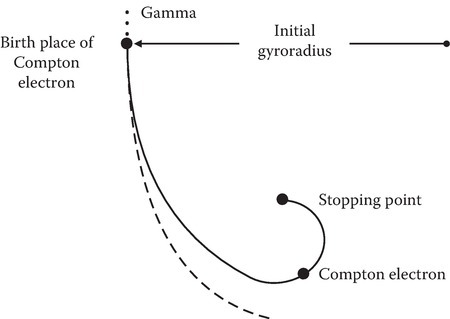
FIGURE 13.24
Birth and turning of the Compton electron in a geomagnetic field.

The secondary electrons have randomly distributed velocities and by themselves do not produce a current. However, in the presence of an electric field, they drift, and this effect is best modeled by Ohm’s law J = σE. The conductivity varies with time with an initial zero value. The current J_c produced by the Compton electrons is in opposition to the conduction current due to the secondary electrons produced by the Compton electrons being stopped by the increasingly dense atmosphere as the gammas travel downwards.

One can use a planar geometry model (Figure 13.25) to approximately calculate and describe the shape of the HEMP-E1.

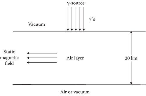
FIGURE 13.25
Planar geometry to simulate E1 HEMP.

Let

(13.224)

$E = \overset{⌢}{x} E_{x} (T)$

(13.225)

$T = t - \frac{z}{c} .$

Thus, E_x is the electric field an observer at z would see if the person “triggered the horizontal sweep on the arrival of the gamma pulse” [25]. However, the field E_x(T, z) will be the electric field observed by different observers (distinguished by their z coordinates) on their gamma-triggered scopes.

The outgoing wave equation for the simplified planar model is given by Longmire [25] from the conservation of the energy principle:

(13.226)

$\frac{\partial E_{x}}{\partial z} + \frac{η_{0} σ}{2} E_{x} = - \frac{η_{0}}{2} J_{c x} .$

If there is no Compton current (J_cx = 0), then E_x attenuates with distance according to

(13.227)

$E_{x} (T, z) = E_{x 0} (T) e^{- \frac{η_{0} σ}{2} z} .$

On the other hand, the very early-time approximation will be based on the conductivity being negligible, and the electric field is entirely due to the Compton current and is given by

(13.228)

$E_{x} (T, z) = - \frac{η_{0}}{2} \int_{0}^{z} J_{c x} (T, z^{'}) d z^{'} .$

Based on these approximations, one can deduce that the shape of the pulse will be as shown by the solid line in Figure 13.26. A qualitative explanation for the shape is as follows.

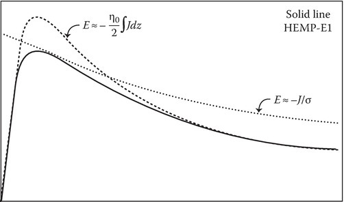
FIGURE 13.26
The broken line curve is the electric field due to the Compton current and the dotted line curve is due to saturation. The solid line curve is the HEMP-E1.

The electromagnetic pulse is due to the two competing effects: the Compton current generating the electric field as per (13.228), shown as a broken line curve in Figure 13.26, and the secondary electrons making conductivity that tries to quench the electric field.

This leads to an effect called saturation [26], shown in Figure 13.26 as a dotted curve, which will not permit the electric field to become too high. The peak value for the electric field will increase with the fast buildup of E1 by Compton current and also will increase with the slow buildup of the conductivity by the secondary electrons. The peak value is less dependent on the yield of the nuclear blast than on the relative rates of E1 buildup due to Compton electrons, and the buildup of the conductivity due to the secondary electrons. The later buildup depends on the air chemistry as discussed in [26].

A mathematical expression [26] for a generic waveform of HEMP-E1 given by International Electrotechnical Commission (IEC) is given in (13.229):

(13.229a)

$E_{1} (t) = 0, t < 0$

(13.229b)

$E_{1} (t) = E_{01} k_{1} (e^{- b_{1} t} - e^{- a_{1} t}), t > 0$

(13.229c)

$E_{01} = 50 kV m^{- 1} k_{1} = 1.3 a_{1} = 6 \times 10^{8} s^{- 1} b_{1} = 4 \times 10^{7} s^{- 1} .$

The peak value is about 73,500 times the amplitude of a typical FM signal. A vast amount of information is available on the topic of the HEMP, and two additional references [27,28] are chosen to lead to some of them.

An electrical circuit analogy to the EMP production is offered in Figure 13.27.

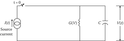
FIGURE 13.27
Circuit analogy to show the competing effects of the Compton electron current flowing through the capacitor and the saturation effect due to the current flow in the voltage-dependent conductance element in parallel. The source current decays with time.

A problem at the end of the chapter pursues this analogy in explaining the competing processes in determining the peak value of the HEMP-E1 and the time of its occurrence.

13.8Magnetohydrodynamics (MHD)

MHD is the science of the interaction of the electric and magnetic fields with a moving conducting fluid. Electric fields arise due to the motion of the conducting fluid in the presence of a magnetic field. The electric field drives a current, which in turn modifies the B field. The mechanical motion of the system is described in terms of the hydrodynamic variables ρ (mass density), v (velocity), and p (pressure), and the electromagnetic variables E, B, and J. The relevant equations are [15,17]

(13.230)

$\frac{\partial ρ}{\partial t} + \nabla \cdot (ρ v) = 0$

(13.231)

$ρ \frac{d v}{d t} = - \nabla p + J \times B + F_{v} + ρ g$

(13.232)

$\nabla \times E = - \frac{\partial B}{\partial t}$

(13.233)

$\nabla \times B = μ_{0} J .$

In Equation 13.231, F_v is the viscous force. In Equation 13.233 we did not include the term due to the displacement current, since it is much smaller than the term due to the conduction current for most of the MHD applications.

A simplified constitutive equation (Ohm’s law) for this case is given by

(13.234)

$J = σ (E + v \times B) .$

Equation 13.234 can be obtained by noting that in the rest frame moving with nonrelativistic velocity v, J′ = σE′ and J = J′ + ρ_ev. But ρ_e, the net charge density, is zero, since in this one component model, both ions and electrons move with the same velocity and there is no charge accumulation. Thus, J = J′. However,

(13.235)

$E^{'} = (E + v \times B) .$

For some applications, instead of (13.234), one may have to use a more generalized Ohm’s law [15].

13.8.1Evolution of the B Field

In MHD applications, the study of the evolution of the B field by itself is important.

From (13.232) and (13.234),

(13.236)

$\frac{\partial B}{\partial t} = - \nabla \times E = - \nabla \times [\frac{J}{σ} - v \times B]$

(13.237)

$\frac{\partial B}{\partial t} = - \nabla \times [\frac{\nabla \times B}{σ μ_{0}}] + \nabla \times (v \times B)$

(13.238)

$\frac{\partial B}{\partial t} = - \frac{1}{σ μ_{0}} [\nabla (\nabla \cdot B) - \nabla^{2} B] + \nabla \times (v \times B) .$

Since ∇ ⋅ B is zero, the equation for B can be written as

(13.239)

$\frac{\partial B}{\partial t} = ν_{m} \nabla^{2} B + \nabla \times (v \times B),$

where ν_m is called magnetic viscosity given by

(13.240)

$ν_{m} = \frac{1}{σ μ_{0}} .$

The first term on the RHS of (13.239) is called the diffusion term, and the second term is called the flow term.

The behavior of the solution of (13.239) largely depends on the conductivity σ. Let us study the effect of each term on the RHS of (13.239) on the solution for B.

Case 1 (v = 0) fluid at rest

For the case of the fluid at rest, B satisfies the following equation:

(13.241)

$\frac{\partial B}{\partial t} = ν_{m} \nabla^{2} B .$

Equation 13.241 is a classical diffusion equation showing that an initial configuration of B vector will decay away in a diffusion time τ_d. The expression for the τ_d can be obtained as follows. If L is a characteristic length, then (13.241) may be approximated as

(13.242)

$\frac{\partial B}{\partial t} \approx \frac{ν_{m}}{L^{2}} B$

and its solution as

(13.243)

$B \approx B_{0} e^{- \frac{ν_{m}}{L^{2}} t} = B_{0} e^{- \frac{t}{τ_{d}}},$

where

(13.244)

$τ_{d} = \frac{L^{2}}{ν_{m}} = σ μ_{0} L^{2} .$

Based on (13.244), it is estimated [17] that it takes 10⁴ years for the magnetic field to decay in the molten core of the earth and 10¹⁰ years in the sun.

Case 2 σ large

The other limit is that sigma is large, and thus, ν_m is small. One can quantify how small it needs to be by defining the magnetic Reynolds number R_m:

(13.245)

$R_{m} = \frac{v L}{ν_{m}} = \frac{v τ_{d}}{L} .$

The Case 2 belongs to the high Reynolds number. In this case, the first term in (13.239) is neglected and the equation for B vector is given by

(13.246)

$\frac{\partial B}{\partial t} = \nabla \times (v \times B) .$

Integrating (13.246) over an open surface S

(13.247)

$\iint_{S} \frac{\partial B}{\partial t} \cdot d s = \iint_{S} \nabla \times (v \times B) \cdot d s = \oint_{C} (v \times B) \cdot d l = - \oint_{C} (B) \cdot (v \times d l) .$

Thus, we have

(13.248)

$\iint_{S} \frac{\partial B}{\partial t} \cdot d s + \oint_{C} (B) \cdot (v \times d l) = 0.$

The LHS of (13.248) can be combined into one term [15] giving us

(13.249)

$\frac{d}{d t} \int_{S} B \cdot d s = 0.$

Equation 13.249 states that the magnetic flux passing through the moving surface stays constant. This is known as the “frozen field condition.”

The proof that (13.249) can be obtained from (13.248) is given as a problem since such a proof helps to understand the emf calculation by transformer emf and motional emf stated in (1.61) of Section 1.6.

13.9Time-Varying Electromagnetic Medium

In Section 13.6.8, under photon ray theory, we considered space and time refraction separately and showed that a temporal discontinuity in the properties of a medium causes a change in the frequency. In this section, we briefly discuss the theory and applications of this frequency-shifting property of a time-varying medium from the viewpoint of full wave theory and Maxwell’s equations. A more extensive discussion, particularly the aspect of amplitude calculations of the newly created frequency-shifted waves, is given in Kalluri [21].

13.9.1Frequency Change due to a Temporal Discontinuity in the Medium Properties

Let us consider normal incidence on a spatial discontinuity in the dielectric properties of a medium of a plane wave propagating in the z-direction. The spatial step profile of the permittivity ε is shown at the top of Figure 13.28a.

FIGURE 13.28
Comparison of the effects of (a) spatial and (b) temporal discontinuities.

The permittivity suddenly changes from ε₁ to ε₂ at z = 0. Let us also assume that the permittivity profile is time invariant. The phase factors of the incident, reflected, and transmitted waves are expressed as $ψ_{A} = e^{j (ω_{A} t - k_{A} z)}$ , where the subscript A = I for the incident wave, A = R for the reflected wave, and A = T for the transmitted wave. The boundary condition of the continuity of the tangential component of the electric field at z = 0 for all t requires

(13.250)

$ω_{I} = ω_{R} = ω_{T} = ω_{A} .$

This result can be stated as follows: The frequency ω is conserved across a spatial discontinuity in the properties of the electromagnetic medium. As the wave crosses from one medium to the other in space, the wave number k changes as dictated by the change in the phase velocity, not considering absorption here. The bottom part of Figure 13.28a illustrates this aspect graphically. The slopes of the two straight lines in the ω−k diagram are the phase velocities in the two mediums. Conservation of ω is implemented by drawing a horizontal line, which intersects the two straight lines. The k values of the intersection points give the wave numbers in the two mediums.

A dual problem can be created by considering a temporal discontinuity in the properties of the medium. Let an unbounded medium (in space) undergo a sudden change in its permittivity at t = 0. The continuity of the electric field at t = 0 now requires that the phase factors of the wave existing before the discontinuity occurs, called a source wave, must match with phase factors, Ψ_N, of the newly created waves in the altered or switched medium, when t = 0 is substituted in the phase factors. This must be true for all values of z. Thus, it leads to the requirement that k is conserved across a temporal discontinuity in a spatially invariant medium. Conservation of k is implemented by drawing a vertical line in the ω−k diagram as shown in the bottom part of Figure 13.28b. The ω values of the intersection points give the frequencies of the newly created waves [29,30,31,32].

13.9.2Effect of Switching an Unbounded Isotropic Plasma Medium

Wave propagation in isotropic plasmas is discussed in Chapter 9. Given below is a summary to act as a self-supporting background of this topic in reference to the time-varying media topic under discussion here.

Any plasma is a mixture of charged particles and neutral particles. The mixture is characterized by two independent parameters for each of the particle species. These are the particle density N and the temperature T. There is a vast amount of literature on plasmas. A few references of direct interest to the reader of this chapter are provided in [15,33,34]. The models are adequate in exploring some of the applications where the medium can be considered to have time-invariant electromagnetic parameters.

There are some applications in which the thermal effects are unimportant. Such a plasma is called cold plasma. A Lorentz plasma [33] is a further simplification of the medium. It is assumed that the electrons interact with each other in a Lorentz plasma only through collective space charge forces and that the heavy positive ions and neutral particles are at rest. The positive ions serve as a background that ensures the overall charge neutrality of the mixture. In this section, the Lorentz plasma is the dominant model used to explore the major effects of a nonperiodically time-varying electron density profile N(t).

The constitutive relations for this simple model viewed as a dielectric medium are given by

(13.251)

$D = ε_{o} ε_{p} E,$

where

(13.252)

$ε_{p} = 1 - \frac{ω_{p}^{2}}{ω^{2}},$

and

(13.253)

$ω_{p}^{2} = \frac{q^{2} N}{m ε_{o}} .$

In these equations, q and m are the absolute values of the charge and mass of the electron, respectively, and $ω_{p}^{2}$ is the square of the plasma frequency proportional to the electron density.

A sketch of ε_p versus ω is given in Figure 9.1. The relative permittivity ε_p is real-positive valued only if the signal frequency is larger than the plasma frequency. Hence, ω_p is a cutoff frequency for the isotropic plasma. Above cutoff, a Lorentz plasma behaves as a dispersive dielectric with the relative permittivity lying between 0 and 1.

The relative permittivity of the medium can be changed by changing the electron density N, which in turn can be accomplished by changing the ionization level. The sudden change in the permittivity shown in Figure 13.28b is an idealization of a rapid ionization. Quantitatively, the sudden-change approximation can be used if the period of the source wave is much larger than the rise time of the temporal profile of the electron density (subcycle time–varying medium). A step change in the profile is referred to in the literature as sudden creation [21,30] or flash ionization [21].

Experimental realization of a small rise time is not easy. A large region of space has to be ionized uniformly at a given time. Joshi et al. [35], Kuo [36], Kuo and Ren [37], as well as Rader et al. [38] developed ingenious experimental techniques to achieve these conditions and demonstrated the principle of frequency shifting using isotropic plasma (see Part IV of Reference 21). One of the earliest pieces of experimental evidence of frequency shifting quoted in the literature is a seminal paper by Yablonovitch [39]. Savage et al. [40] used the ionization front to upshift the frequencies. Ionization front is a moving boundary between unionized medium and the plasma [41]. Such a front can be created by a source of ionizing radiation pulse, say, a strong laser pulse. As the pulse travels in a neutral gas, it converts it into plasma, thus creating a moving boundary between the plasma and the unionized medium. However, the ionization-front problem is somewhat different from the moving-plasma problem. In the front problem, the boundary alone is moving and the plasma is not moving with the boundary.

The constitutive relation (13.251), based on the dielectric model of a plasma, does not explicitly involve the current density J in the plasma. The constitutive relations that involve the plasma current density J are given by

(13.254)

$D = ε_{o} E,$

(13.255)

$J = - q N v .$

The velocity v of the electrons is given by the force equation

(13.256)

$m \frac{d v}{dt} = - q E .$

In (13.256), the magnetic force due to the wave’s magnetic field H is neglected since it is much smaller [33] than the force due to the wave’s electric field. The magnetic force term (−qv × H) is nonlinear. Stanic [42] studied this problem as a weakly nonlinear system.

Since ion motion is neglected, (13.255) does not contain ion current. Such an approximation is called radio approximation [34]. It is used in the study of radio wave propagation in the ionosphere. Low-frequency wave propagation studies take into account the ion motion [34].

Substituting (13.254), (13.255) and (13.256) in the Ampere–Maxwell equation

(13.257)

$\nabla \times H = J + \frac{\partial D}{\partial t},$

we obtain

(13.258)

$\nabla \times H = j ω ε_{o} ε_{p} (ω) E,$

where ε_p(ω) is given by (13.252) and an exp(jωt) time dependence has been assumed. For an arbitrary temporal profile of the electron density N(t), (13.255) is not valid [21,43,44]. The electron density N(t) increases because of the new electrons born at different times. The newly born electrons start with zero velocity and are subsequently accelerated by the fields. Thus, all the electrons do not have the same velocity at a given time during the creation of the plasma. Therefore,

(13.259)

$J (t) \neq - q N (t) v (t),$

but

(13.260)

$Δ J (t) = - q Δ N_{i} v_{i} (t),$

instead. Here, ΔN_i is the electron density added at t_i, and v_i(t) is the velocity at time t of these ΔN_i electrons born at time t_i. Thus, J(t) is given by the integral of (13.260) and not by (13.259). The integral of (13.260), when differentiated with respect to t, gives the constitutive relation between J and E as follows:

(13.261)

$\frac{d J}{d t} = ε_{o} ω_{p}^{2} (r, t) E (r, t) .$

Equations 13.257 and 13.261 and the Faraday equation

(13.262)

$\nabla \times E = - μ_{o} \frac{\partial H}{\partial t}$

are needed to describe the electromagnetics of isotropic plasmas.

Propagation of an electromagnetic wave traveling in the z-direction with $E = \hat{x} E$ and $H = \hat{y} H$ can be studied by assuming that the components of the field variables have harmonic space variation, that is,

(13.263)

$F (z, t) = f (t) e^{- j k z} .$

Substituting (13.263) in (13.257), (13.261), and (13.262), we obtain the wave equations

(13.264)

$\frac{d^{2} E}{d t^{2}} + [k^{2} c^{2} + ω_{p}^{2} (t)] E = 0,$

and

(13.265)

$\frac{d^{3} H}{d t^{3}} + [k^{2} c^{2} + ω_{p}^{2} (t)] \frac{d H}{d t} = 0,$

for E and H.

13.9.2.1Sudden Creation of an Unbounded Plasma Medium

The geometry of the problem is shown in Figure 13.29. A plane wave of frequency ω_o is propagating in free space in the z-direction. Suddenly at t = 0, an unbounded plasma medium of plasma frequency ω_p is created. Thus arises a temporal discontinuity in the properties of the medium. The solution of (13.265), when ω_p is a constant, can be obtained as

(13.266)

$H (t) = \sum_{m = 1}^{3} H_{m} exp (j ω_{m} t),$

where

(13.267)

$ω_{m} [ω_{m}^{2} - (k^{2} c^{2} + ω_{p}^{2})] = 0.$

The ω−k diagram [2] for the problem under discussion is obtained by graphing (13.267). Figure 13.30 shows the ω−k diagram, where the top and the bottom branches are due to the factor in the square brackets equated to zero, and the horizontal line is due to the factor ω = 0. The line k = constant is a vertical line that intersects the ω−k diagram at the three points marked as 1, 2, and 3. The third mode is the wiggler mode [21,30,45]. Its real-valued fields are

(13.268)

$E_{3} (x, y, z, t) = 0,$

(13.269)

$H_{3} (x, y, z, t) = \hat{y} H_{o} \frac{ω_{p}^{2}}{ω_{o}^{2} + ω_{p}^{2}} cos (k z),$

(13.270)

$J_{3} (x, y, z, t) = \hat{x} H_{o} k \frac{ω_{p}^{2}}{ω_{o}^{2} + ω_{p}^{2}} sin (k z) .$

It is of zero frequency but varies in space. Such wiggler fields are used in a free electron laser (FEL) to generate coherent radiation [46]. Its electric field is zero but has a magnetic field due to the plasma current J₃. In the presence of a static magnetic field in the z-direction, the third mode becomes a traveling wave with a downshifted frequency. This aspect is discussed below in Section 13.9.4, under Frequency-shifting characteristics of various R waves.

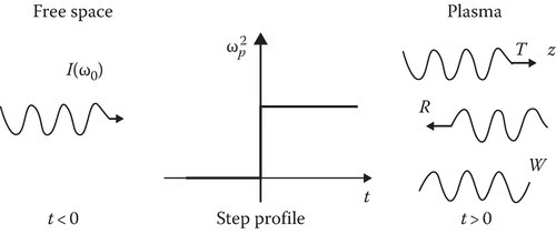
FIGURE 13.29
Suddenly created unbounded plasma medium.

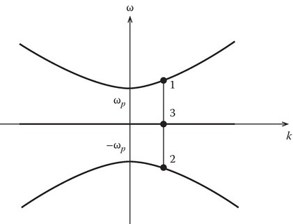
FIGURE 13.30
ω−k diagram and wiggler magnetic field.

The modes 1 and 2 have frequencies given by

(13.271)

$ω_{1, 2} = \pm \sqrt{(ω_{p}^{2} + k^{2} c^{2})},$

where ω₂ has a negative value. Since the harmonic variations in space and time are expressed in the phase factor exp(ω t − kz), a negative value for ω gives rise to a wave propagating in the negative z-direction. It is a backward-propagating wave or, for convenience, can be referred to as a wave reflected by the discontinuity. The modes 1 and 2 have higher frequencies than the source wave. These are upshifted waves.

13.9.3Sudden Creation of a Plasma Slab

The interaction of an electromagnetic wave with a plasma slab is experimentally more realizable than with an unbounded plasma medium. When an incident wave enters a pre-existing plasma slab, the wave must experience a spatial discontinuity. If the plasma frequency is lower than the incident wave frequency, then the incident wave is partially reflected and transmitted. When the plasma frequency is higher than that of the incident wave, the wave is totally reflected because the relative permittivity of the plasma is less than zero.

However, if the plasma slab is sufficiently thin, the wave can be transmitted by tunneling effect [21]. For this time-invariant plasma, the reflected and transmitted waves have the same frequency as the source wave frequency, and they are called as A waves. The wave inside the plasma has a different wave number but the same frequency due to the requirement of the boundary conditions.

When a source wave is propagating in free space and suddenly a plasma slab is created, the wave inside the slab region experiences a temporal discontinuity in the properties of the medium. Hence, the switching action generates new waves whose frequencies are upshifted, and then the waves propagate out of the slab. They are called as B waves. The phenomenon is illustrated in Figure 13.31a. In Figure 13.31a, the source wave of frequency ω_o is propagating in free space. At t = 0, a slab of plasma frequency ω_p is created. The A waves in Figure 13.31b have the same frequency as that of the source wave. The B waves are newly created waves due to the sudden switching of the plasma slab and have upshifted frequencies $ω_{1} = \sqrt{(ω_{o}^{2} + ω_{p}^{2})} = - ω_{2}$ . The negative value for the frequency of the second B wave shows that it is a backward-propagating wave. These waves, however, have the same wave number as that of the source wave as long as they remain in the slab region. As the B waves come out of the slab, they encounter a spatial discontinuity, and therefore the wave number changes accordingly. The B waves are only created at the time of switching and, hence, exist for a finite time. In Figure 13.31, the waves are sketched in the time domain to show frequency changes. Thus, the arrow head symbol in the sketches show the t variable. See Figure 13.31b for a more accurate description. Note that the vertical axis is ct.

FIGURE 13.31
Effect of switching an isotropic plasma slab. A waves have the same frequency as the incident wave frequency (ω_o), and B waves have upshifted frequency $ω_{1} = \sqrt{(ω_{o}^{2} + ω_{p}^{2})} = - ω_{2}$ . (a) The waves are sketched in the time domain to show the frequency changes. (b) Shows a more accurate description.

13.9.4Time-Varying Magnetoplasma Medium

Wave propagation in an anisotropic magnetoplasma is discussed in Chapter 11. Given below is a summary to act as a self-supporting background of this topic in reference to the time-varying media topic under discussion here.

A plasma medium in the presence of a static magnetic field behaves like an anisotropic dielectric [21]. Therefore, the theory of electromagnetic wave propagation in this medium is similar to the theory of light waves in crystals. Of course, in addition, account has to be taken of the highly dispersive nature of the plasma medium.

A cold magnetoplasma is described by two parameters: the electron density N and the quasistatic magnetic field. The first parameter is usually given in terms of the plasma frequency ω_p. The strength and the direction of the quasistatic magnetic field have significant effect on the dielectric properties of the plasma. The parameter that is proportional to the static magnetic field is the electron gyrofrequency ω_b defined below. The cutoff frequency of the magnetoplasma is influenced by ω_p as well as ω_b. An additional important aspect of the dielectric properties of the magnetoplasma medium is the existence of a resonant frequency. At the resonant frequency, the relative permittivity ε_p goes to infinity. As an example, for longitudinal propagation defined under characteristic waves, resonance occurs when the signal frequency ω is equal to the electron gyrofrequency ω_b. For the frequency band, 0 < ω < ω_b, ε_p > 1 and can have very high values for certain combinations of ω, ω_p, and ω_b; for instance, when $f_{p} = \frac{ω_{p}}{2 π} = 10^{14} Hz$ , $f_{b} = \frac{ω_{b}}{2 π} = 10^{10} Hz$ , and f = 10 cm, ε = 9 × 10¹⁶ [34]. A big change in ε_p can thus be obtained by collapsing the electron density, thus converting the magnetoplasma medium into free space. A big change in ε_p can also be obtained by collapsing the background quasistatic magnetic field, thus converting the magnetoplasma medium into an isotropic plasma medium. These aspects are discussed in the remaining parts of this section.

13.9.4.1Basic Field Equations

The electric field E(r, t) and the magnetic field H(r, t) satisfy the Maxwell curl equations:

(13.272)

$\nabla \times E = - μ_{0} \frac{\partial H}{\partial t},$

(13.273)

$\nabla \times H = ε_{0} \frac{\partial E}{\partial t} + J .$

In the presence of a quasistatic magnetic field B₀, the constitutive relation for the current density is given by

(13.274)

$\frac{d J}{d t} = ε_{0} ω_{p}^{2} (r, t) E - J \times ω_{b} (r, t),$

where

(13.275)

$ω_{b} = \frac{q B_{0}}{m} = ω_{b} {\hat{B}}_{0} .$

Therein, ${\hat{B}}_{0}$ is a unit vector in the direction of the quasistatic magnetic field, ω_b is the gyrofrequency, and

(13.276)

$ω_{p}^{2} (r, t) = \frac{q^{2} N (r, t)}{m ε_{o}} .$

13.9.4.2Characteristic Waves

Next, the solution for a plane wave propagating in the z-direction in a homogeneous, time-invariant unbounded magnetoplasma medium can be obtained by assuming

(13.277)

$f (z, t) = exp [j (ω t - k z)],$

(13.278)

$ω_{p}^{2} (z, t) = ω_{p}^{2},$

(13.279)

$ω_{b} (z, t) = ω_{b},$

where f stands for the components of the field variables E, H, or J.

The well-established magnetoionic theory [33,34] and [15] is concerned with the study of plane wave propagation of an arbitrarily polarized plane wave in a cold, anisotropic plasma, where the direction of phase propagation of the plane wave is at an arbitrary angle to the direction of the static magnetic field. As the plane wave travels in such a medium, the polarization state continuously changes. However, there are specific normal modes of propagation in which the state of polarization is unaltered. Plane waves with left (L wave) or right (R wave) circular polarization are the normal modes in the case of wave propagation along the quasistatic magnetic field. Such propagation is labeled as longitudinal propagation. The ordinary wave (O wave) and the extraordinary wave (X wave) are the normal modes for transverse propagation, where the direction of propagation is perpendicular to the static magnetic field. In this chapter, propagation of the R wave in a time-varying plasma is discussed. An analysis of the propagation of other characteristic waves can be found elsewhere [21].

13.9.4.3R-Wave Propagation

The relative permittivity for R-wave propagation is [21,33]

(13.280)

$ε_{p R} = 1 - \frac{ω_{p}^{2}}{ω (ω - ω_{b})} = \frac{(ω + ω_{c 1}) (ω - ω_{c 2})}{ω (ω - ω_{b})},$

where ω_c1 and ω_c2 are the cutoff frequencies given by

(13.281)

$ω_{c 1, c 2} = \mp \frac{ω_{b}}{2} + \sqrt{{(\frac{ω_{b}}{2})}^{2} + ω_{p}^{2}} .$

Equation 13.280 is obtained by eliminating J from (13.273) with the help of (13.274) and recasting it in the form of (13.258).

The dispersion relation is obtained from

(13.282)

$k_{R}^{2} c^{2} = ω^{2} ε_{p R} = \frac{ω (ω + ω_{c 1}) (ω - ω_{c 2})}{(ω - ω_{b})},$

where k_R is the wave number for the R wave and c is the speed of light in free space. When expanded, this equation becomes

(13.283)

$ω^{3} - ω_{b} ω^{2} - (k_{R}^{2} c^{2} + ω_{p}^{2}) ω + k_{R}^{2} c^{2} ω_{b} = 0.$

Figure 13.32, which is the same as Figure 11.1, shows a graph of ε_p versus ω, while Figure 13.33 gives the ω−k diagram for R-wave propagation. The R wave is a characteristic wave of longitudinal propagation. For this wave, the medium behaves like an isotropic plasma except that ε_p is influenced by the strength of the quasistatic magnetic field. Particular attention is drawn to the specific feature, visible in Figure 13.32, showing ε_p > 1 for the R wave in the frequency band 0 < ω < ω_b. This mode of propagation is called whistler mode in the literature on ionospheric physics and helicon mode in the literature on solid-state plasmas. Section 10C7.6 and 10C7.7 of Reference [22] deal with the transformation of the whistler wave by a transient magnetoplasma medium and the consequences of such a transformation. An isotropic plasma medium does not support a whistler wave.

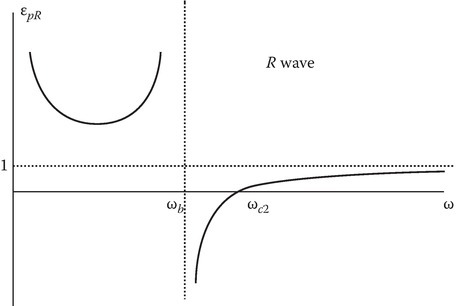
FIGURE 13.32
Relative permittivity for a R-wave propagation.

FIGURE 13.33
ω−k diagram for a R-wave propagation.

13.9.4.4Sudden Creation

In this section, the problem of sudden creation of the plasma in the presence of a static magnetic field in z-direction is analyzed. The geometry of the problem is given in Figure 13.34. The source wave is assumed to be an R wave. The sudden creation is equivalent to creating a temporal discontinuity in the dielectric properties of the medium. In such a case, the wave number k₀ is conserved across the temporal discontinuity. For a given k₀ of the source wave, we draw a vertical line that intersects the branches in the ω−k diagram in Figure 13.33 at three points. The frequencies of these waves are different from the source frequency. The medium switching, in this case, creates three R waves labeled as R₁, R₂, and R₃. Whereas R₁ and R₃ are transmitted waves, R₂ is a reflected wave (Figure 13.34).

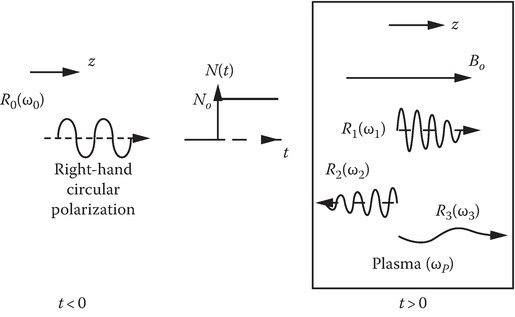
FIGURE 13.34
Effect of switching an unbounded magnetoplasma medium. Sketches of the B waves generated in the plasma are given for R incidence. The waves are sketched in the time domain to show the frequency changes.

A physical interpretation of the waves can be given in the following way: The electric and magnetic fields of the incident wave and the quasistatic magnetic field accelerate the electrons in the newly created magnetoplasma, which in turn radiate new waves. The frequencies of the new waves and their fields can be obtained by adding contributions from the many electrons whose positions and motions are correlated by the collective effects supported by the magnetoplasma medium. Such a detailed calculation of the radiated fields seems to be quite involved. A simple, but less accurate, description of the plasma effect is obtained by modeling the magnetoplasma medium as a dielectric medium whose refractive index is computed through magnetoionic theory [34]. The frequencies of the new waves are constrained by the requirements that the wave number k₀ is conserved over the temporal discontinuity and the refractive index n is the one that is applicable to the type of wave propagation in the magnetoplasma. This gives a conservation law [47] k₀c = ω₀ = n(ω) from which ω can be determined. Solution of the associated electromagnetic initial value problem gives the electric and magnetic fields of the new waves.

13.9.4.5Frequency-Shifting Characteristics of Various R Waves

The shift ratio and the efficiency of the frequency-shifting operation can be controlled by the parameters ω_p and ω_b. The results are presented by normalizing all frequency variables with respect to the source wave frequency ω₀. This normalization is achieved by taking ω₀ = 1 in numerical work.

For R waves, the curves of ω − ω_p and ω − ω_b are sketched in Figure 13.35a and b, respectively. In Figure 13.36, results are presented for the R₁ wave: The values on the vertical axis give a frequency-shift ratio since the frequency variables are normalized with respect to ω₀. This is an upshifted wave and the shift ratio increases with ω_p as well as ω_b. From Figure 13.36 it appears that by a suitable choice of ω_p and ω_b, one can obtain any desired large frequency shift. However, the wave generated can have weak fields associated with it and the power density S₁ can be low. This point is illustrated in Table 13.1 by considering two sets of values for the parameters (ω_p , ω_b). For the set (0.5, 0.5), the shift ratio is 1.2, but the power density ratio S₁/S₀ is 0.57; whereas for the set (2.0, 2.0), the shift ratio is 3.33 but the power density ratio is only 0.07. Similar remarks apply to other waves.

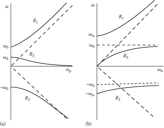
FIGURE 13.35
Frequency shifting of R waves. Sketches of (a) ω versus ω_p, (b) ω versus ω_b; $ω_{is} = {(ω_{o}^{2} + ω_{p}^{2})}^{1 / 2}$ .

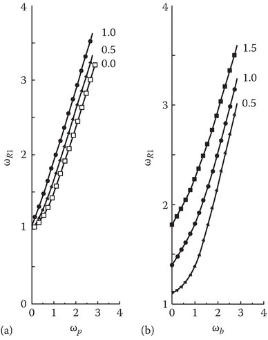
FIGURE 13.36
Frequency shifting of the R₁ wave. The frequency variables are normalized with respect to the source wave frequency by taking ω₀ = 1. Shown is the frequency-shift ratio versus (a) ω_p and (b) ω_b. The numbers on the curves are (a) ω_b and (b) ω_p.

TABLE 13.1
R₁ Wave-Shift Ratio and Power Density for Two Sets of (ω_p, ω_b)

The R₂ wave is a reflected wave. This is an upshifted wave and the shift ratio increases with ω_b but decreases with ω_b [21]. The R₃ wave in Figure 13.37 is a transmitted wave that is downshifted. The shift ratio decreases with ω_p and increases with ω_b. When ω_b = 0, ω_R3 becomes zero. The electric field E₃ becomes zero, and the magnetic field degenerates to the wiggler magnetic field [48]. This result is in conformity with the result for the isotropic case discussed in Section 13.9.2.1.

FIGURE 13.37
Frequency shifting of the R₃ wave. ω₀ = 1. Shown is the frequency-shift ratio versus (a) ω_p and (b) ω_b. The numbers on the curves are (a) ω_b and (b) ω_p.

13.9.5Modeling of Building Up Plasma versus Collapsing Plasma

13.9.5.1Building Up Magnetoplasma

For the case of building-up plasma, the total current density, J(t), cannot simply be taken as –qN(t)v(t) since the electron velocity, v(t), depends on the time of electron birth. The newly born electrons start with zero velocity and are subsequently accelerated by the fields. Thus, all the electrons do not have the same velocity at a given time during the creation or building-up of the plasma. When the electron density is increasing due to electrons born with zero velocity at different times, the change in current density at t due to the electrons born at t_i can be computed as follows [21]:

(13.284)

$Δ J (t) = - q Δ N_{i} v_{i} (t) .$

where ΔN_i is the electron density added at t_i and v_i(t) is the velocity at t of these ΔN_i electrons born at t_i. To obtain J(t), Equation 13.284 must be integrated to account for the current density contributions from electrons born at all times t_i [Appendix A of Reference 21]. This results in the constitutive equation for the plasma creation case:

(13.285)

$\frac{d J}{d t} + ν J = ε_{0} ω_{p}^{2} (r, t) E - J \times ω_{b} (r, t) + \frac{q}{m} \nabla p .$

Here the electron cyclotron frequency (gyrofrequency) ω_b is given by

(13.286)

$ω_{b} = \frac{q B_{0}}{m} = ω_{b} {\hat{B}}_{0},$

where ${\hat{B}}_{0}$ is a unit vector in the direction of the static magnetic field and q and m are the absolute values of the charge and mass of the electron, respectively. The square of the plasma frequency, $ω_{p}^{2}$ , is proportional to the electron density, N(r, t), and given by

(13.287)

$ω_{p}^{2} (r, t) = \frac{q^{2} N (r, t)}{m ε_{0}} .$

The gradient term in (13.285) is to account for the warm plasma case, discussed in Chapter 10.

13.9.5.2Collapsing Magnetoplasma

In the case of collapsing magnetoplasma due to the collapse of the ionization, the building-up plasma formulation of the previous section is not appropriate [21,49,50] because as the plasma decays the number of free electrons decreases, and therefore, ultimately, the current vector density J should disappear. However, using the above model, the collapsing plasma makes dJ/dt = 0 and does not make J = 0 ([21, p. 148] and [49,50]). An alternative model is needed to implement this condition.

One can consider the following model for the collapse of the plasma: the decrease in the electron density takes place by the process of sudden removal of ΔN(t) electrons; the velocities of all the remaining electrons are unaffected by this capture and have the same instantaneous velocity v(t). The model has to ensure the continuity of v(t). The modification of (13.284) for the collapsing plasma is obtained as follows. Since the electrons are assumed to all have the same velocity v(t), the current density is given by

(13.288)

$J (t) = - q N (r, t) v (t) .$

Taking the derivative of (13.288) with respect to time results in

(13.289)

$\frac{d J}{d t} = - q \frac{\partial N (r, t)}{\partial t} v (t) - q N (r, t) \frac{\partial v (t)}{\partial t} .$

Substituting (13.288) and (13.289) into the momentum equation (13.285), and using (13.286) and (13.287) results in the constitutive relation for the collapsing plasma case

(13.290)

$\frac{d J}{d t} + [ν - \frac{\frac{\partial}{\partial t} [ω_{p}^{2} (t)]}{ω_{p}^{2} (t)}] J = ε_{0} ω_{p}^{2} (r, t) E - J \times ω_{b} (r, t) + \frac{q}{m} \nabla p .$

Even if it is assumed that the plasma is loss free (ν = 0), the term involving the time derivative of ω $ω_{p}^{2} (t)$ ensures the current density J ultimately disappears when the plasma collapses completely. The parameter ν in (13.290) represents the energy dissipated as heat, whereas the ${[ω_{p}^{2} (t)]}^{'} / ω_{p}^{2} (t)$ term represents the energy loss due to the ΔN(t) electrons lost in the plasma decay process. Neglecting this term can lead to errors as shown in [50]. If ν₁ is defined as

(13.291)

$\begin{array}{l} ν_{1} = ν building-up plasma \\ ν_{1} = ν - \frac{\frac{\partial}{\partial t} [ω_{p}^{2} (t)]}{ω_{p}^{2} (t)} collapsing plasma . \end{array}$

the constitutive equation for either case can be written as

(13.292)

$\frac{d J}{d t} + ν_{1} J = ε_{0} ω_{p}^{2} (r, t) E - J \times ω_{b} (r, t) + \frac{q}{m} \nabla p .$

The pressure p can also be related to the electric field E by the following equation [22]:

(13.293)

$\nabla p = - γ k_{B} T \frac{ε_{0}}{q} \nabla (\nabla \cdot E),$

and equation (13.292) can be written as

(13.294)

$\frac{d J}{d t} + ν_{1} J = ε_{0} ω_{p}^{2} (r, t) E - J \times ω_{b} (r, t) - ε_{0} a^{2} \nabla (\nabla \cdot E),$

where

γ is the ratio of specific heats

k_B is the Boltzmann constant [1.38066 × 10⁻²³ J/K]

T is the temperature [K]

ε₀ is the permittivity of free space [8.85418782 × 10⁻¹² F/m]

a is the acoustic velocity [m/s]

The acoustic velocity (a) is given by

(13.295)

$a = {(\frac{γ k_{B} T}{m})}^{\frac{1}{2}} .$

Several interesting results are presented using this model [51].

13.9.6Applications

Many applications for the frequency-shifting research are developing. An obvious application is for frequency transformers. The source wave can be generated in a frequency band using standard equipment, and the switched plasma device converts the source wave into a new wave in a frequency band not easily accessible by other methods. The frequency-shifting mechanism can be applied for plasma cloaking of satellites and aircrafts and for producing short-chirped pulses as ultra-wideband signals [55]. Application to photonics has been dealt in detail by Nerukh et al. [56]. One particular application of great significance is mentioned next.

13.9.6.1Application: Frequency Transformer 10–1000 GHz

An application of the phenomena of frequency upshifting (by a ratio of 100) of a source wave of 10–1000 GHz by a collapsing magnetoplasma in a cavity is discussed in Appendix 13C. The material developed in Sections 13.9.4 and 13.9.5 supplies the background material that will help in understanding the details omitted in Appendix 13C.

As explained before, the interaction of an electromagnetic wave with a time-varying medium is governed by the property of conservation of the wave number. This property can be utilized to construct a frequency transformer. It is shown that switching off the ionization source and creating a decaying magnetoplasma medium in a cavity will upshift the source frequency of 10–1000 GHz for the appropriate choice of initial magnetoplasma parameters. The electric field of the output wave is comparable to that of the source wave. Moreover, the switching angle can alter the polarization of the output wave.

One of the examples given in Appendix 13C has the following parameters: f₀ = 10 GHz, f_p0 = 30 GHz, and f_b = 10.009 GHz, and a plate separation in the cavity of d = 0.15 mm. When the ionization source is switched off, the output mode has a frequency of 1000 GHz. The electric field of the output wave is comparable to the input wave.

The results presented as FDTD solution of this ideal problem has one puzzling aspect: If the frequency of the wave changes from 10 to 1000 GHz, it will go through the cyclotron resonance at f = f_b = 10.009 GHz, should there not be a strong absorption, when the plasma is assumed lossy. The simulation results do not show any such strong absorption even for ν/ω_p = 0.1. A more detailed picture of the variation of the amplitudes and frequencies of the three modes with the decaying plasma parameter ω_p(t) will clarify the results. The interesting physics is explained in Figure 13C.12, which shows the variation of the frequency (a) and the amplitude (b) of the electric field of the three modes labeled as R₁, R₂, and R₃ (for each of the initial components of the standing wave). As ω_p decreases and becomes zero, ω₁ becomes n₀ω₀, ω₂ becomes −n₀ω₀, and ω₃ becomes ω_b.

The puzzle is now solved. At the instant of switching off the plasma, that is at t = 0+, the three modes are excited; the first mode has frequency higher than n₀ω₀, but the amplitude of the electric field is zero. The amplitude builds up as ω_p and decreases reaching a final value E_f. Mode 2 is a negative-going wave but otherwise has similar characteristics as mode 1 and builds up as the plasma collapses. Mode 3 is a positive-going wave with an initial frequency ω₀ and amplitude E₀ of the source R wave. However, as plasma decays, ω₃ increases from ω₀ to ω_b and E₃ amplitude decreases from E₀ to 0. Even if we assume no losses in the plasma medium, this mode dies. In the presence of collisions, it is absorbed at a faster rate. The absorption in this case serves a useful purpose in removing the unwanted mode 3.

The presence of a cavity introduces the switching angle ϕ₀ as a controlling parameter, controlling the relative amplitudes and phases of the x and y components of the electric fields of the output wave. The polarization of the output wave can be altered by changing the switching angle. Figure 13C.11 shows that the output wave is linearly x-polarized for an initial switching angle of ϕ₀ = 90°. However, if the switching angle is zero degrees, the output wave will be y-polarized. Thus the case under study for the chosen parameters (see Figure 13C.11) gives a frequency and polarization transformer, transforming 10 GHz input wave to 1000 GHz output wave with a change of polarization from right circularly polarized to x-polarized.

13.9.7Subcycle Time-Varying Medium

In Sections 13.9.2.1 and 13.9.4.4, we modeled the fast temporal change in the parameters as sudden switching to simplify the problem. In case the rise or decay time is not zero, we can calculate the scattering coefficients by using perturbation and variational techniques to obtain the corrections. Their validity is based on the rise or decay time being small compared to the period of the source wave. The time-varying medium under these restrictions is recognized in [52] as a “subcycle time-varying medium.” A fundamental difference is the requirement of causality in the case of the time-varying medium [21]. A related technique, “comparison identities,” is used to calculate the amplitudes [53,54,55,56].

13.9.8Periodically Time-Varying Parameter, Mathieu Equation, and Parametric Resonance

Equation 13.264, when kc is the signal frequency ω₀ in free space for t < 0, can be written as

(13.296a)

$\frac{d^{2} E}{d t^{2}} + ω^{2} (t) E = 0$

(13.296b)

$ω^{2} (t) = [ω_{0}^{2} + ω_{p}^{2} (t)] .$

It is a linear equation but in general not exactly solvable for a general temporal profile $ω_{p}^{2} (t)$ , in which case it is called Hill’s equation [57]. If the profile is periodic, given by

(13.297a)

$ω_{p}^{2} (t) = ω_{p 0}^{2} cos ω_{x} t,$

Equation 13.296b becomes

(13.297b)

$ω^{2} (t) = ω_{0}^{2} [1 + X cos ω_{x} t],$

where

(13.297c)

$X = \frac{ω_{p 0}^{2}}{ω_{0}^{2}} .$

Equation 13.296a, when (13.297b) is inserted for ω²(t) is called Mathieu equation [58]. For X ≪ 1, small amplitude oscillation at the frequency ω₀ grows in amplitude exponentially in time if ω_x is close to 2ω₀/n, where n is a positive integer. This phenomenon is called parametric resonance [16,57,58,59,60,61,62,63], since it occurs due to the periodic variation of a parameter. The amplitude is most strong when n = 1. Parametric resonance is known to occur in various physical processes. A parametric pendulum, where the pivot of a simple frictionless pendulum is subjected to an alternating vertical motion as shown in Figure 13.38, is discussed in [58].

FIGURE 13.38
Geometry for parametric pendulum.

An L-R-C circuit with a periodically time-varying capacitor (Figure 13.39)

(13.298)

$C (t) = C_{0} [1 + a cos ω_{a} t]$

is discussed in [59].

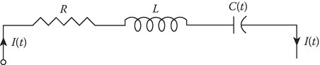
FIGURE 13.39
A series *L-R-C* circuit with a periodically time-varying capacitor.

The differences between forced resonance phenomena and the parametric resonance need to be carefully noted. The equation for the forced resonance is of the canonical form

(13.299)

$\frac{d^{2} E}{d t^{2}} + ω_{0}^{2} E = E_{0} cos ω_{d} t .$

In the forced resonance case, the source frequency ω_d is tuned to the natural frequency of the resonance ω₀. In the parametric resonance case, it is the tuning of the frequency of the time-varying parameter ω_x = 2ω₀/n to the frequency of the source ω₀ that brings resonance. In the forced resonance case, the buildup of the amplitude of oscillation diverges linearly with time, whereas in the case of the parametric resonance, the buildup of the amplitude diverges exponentially with time [59].

The interesting features of the solution of Mathieu’s equation is shown in [58] through the example of a parametric pendulum (Figure 13.38).

The Mathieu equation solved for the pendulum angle θ is

(13.300)

$\frac{d^{2} θ}{d t^{2}} + ω_{0}^{2} [1 + h cos (2 ω t)] θ = 0.$

The forcing term in this case is of amplitude h and period T_exc = 2π/2ω, and the natural period T_nat of the pendulum is 2π/2ω₀. Because of the periodic parameter in (13.300), Floquet’s theorem, discussed in Section 9.7, applies and

(13.301)

$θ (t + T) = e^{μ T} θ (t) .$

The above can be interpreted as the following: Theta gets rescaled by e^{μ^T} each period. The solution of (13.300), Mathieu equation, will be the product of exponential growth/decay term and a periodic function of time. Note that $θ = \dot{θ} = 0$ is a rest state of (13.300), but it is an unstable state if μ is positive. The instability is strongest when the excitation frequency ω in (13.300) is twice the natural frequency ω₀ of the pendulum. One can investigate this instability by taking

(13.302)

$ω = 2 ω_{0} + ε, ε ≪ 1.$

Assuming the excitation amplitude h as small, the solution of (13.300) with ω as given in (13.302) can be written as

(13.303)

$θ (t) = a (t) cos (ω_{0} + \frac{ε}{2}) + b (t) sin (ω_{0} + \frac{ε}{2}) .$

Substituting (13.303) in (13.300), retaining terms that are first order in ε and neglecting second-order derivatives of a and b [58], we can show that

(13.304)

$μ^{2} = \frac{1}{4} [{(\frac{1}{2} h ω_{0})}^{2} - ε^{2}] .$

Parametric resonance occurs when μ is real and positive, which gives the bounds for the relation between ε and h:

(13.305)

$- \frac{1}{2} h ω_{0} < ε < \frac{1}{2} h ω_{0} .$

The inequality relation (13.305) means that the parametric resonance takes place not only when ε is zero but also slightly away from the resonance within the region specified by the two straight lines in the ε − h phase diagram with a slope of ±hω₀/2.

The limit to the amplitude of the parametric oscillation arises due to the damping γ- term in the modified Mathieu equation given below:

(13.306)

$\frac{d^{2} θ}{d t^{2}} + 2 γ \frac{d θ}{d t} + ω_{0}^{2} [1 + h cos ((2 ω_{0} + ε) t)] θ = 0.$

In this case, the inequality relation (13.305) gets modified to

(13.307)

$- {[{(\frac{1}{2} h ω_{0})}^{2} - 4 γ^{2}]}^{\frac{1}{2}} < ε < {[{(\frac{1}{2} h ω_{0})}^{2} - 4 γ^{2}]}^{\frac{1}{2}} .$

Also, the parametric resonance is possible only if h > h_c, where

(13.308)

$h_{c} = \frac{4 γ}{ω_{0}} .$

The above is a brief account of an insightful explanation of the parametric pendulum given in [58]. It is available for free download on the Internet, from which one can obtain more details. Reference [59], also available for free downloading from the Internet, has simulations to show the difference between forced resonance and parametric resonance through an L-C-R-example. Reference [57] has a good account of various physical phenomena of self-oscillation, which sometimes is wrongly attributed to either forced resonance or parametric resonance. Swanson [63] and Chen [16] discuss parametric instabilities in plasmas.

13.10Statistical Mechanics and Boltzmann Equation

Boltzmann equation [15,16,33,64,65,66] is a PDE for a particle distribution function f used to describe particle trajectories in “phase space.” The phase space is a six-dimensional space that consists of both physical space (also called configuration space) denoted by d³x and velocity space denoted by d³v. In the terminology of probability theory, f will be called a density function.

The expression [64]

(13.309)

$f (r, v, t) d^{3} x d^{3} v$

will denote the number of particles located in the phase space between (r, v) and (r + dr, v + dv). The variable N(r, t), the number of particles per unit volume of physical space, can be written as

(13.310)

$N (r, t) = \int f (r, v, t) d^{3} v .$

The limits of integration when not specified are assumed to be over all possible values of velocities in the velocity volume space.

The RHS of (13.310) assumes a simpler form for an isotropic distribution function, that is,

(13.311)

$f (r, v, t) = f (r, v^{2}, t) .$

In such a case we can write (13.310) as

(13.312)

$N (r, t) = 4 π \int_{v = 0}^{\infty} f (r, v^{2}, t) v^{2} d v .$

The above is obtained by writing the differential volume element d³v in velocity space as

(13.313)

$d^{3} v = v^{2} d v sin θ d θ d ϕ .$

Combining the terms that depend on the scalar velocity variable, we can define a new distribution function g:

(13.314)

$g (r, v^{2}, t) = 4 π v^{2} f (r, v^{2}, t) . (1 c 4)$

Note that the function g is zero at v = 0 and attains its maximum elsewhere [16].

If f is normalized so that $\overset{⌢}{f}$

(13.315)

$\int_{- \infty}^{\infty} \overset{⌢}{f} (r, v, t) d^{3} v = 1,$

then

(13.316)

$f (r, v, t) = N (r, t) \overset{⌢}{f} (r, v, t) .$

13.10.1Maxwell Distribution ${\overset{⌢}{f}}_{M}$ and Kinetic Definition of Temperature T

An often used simple example of $\overset{⌢}{f}$ is called the Maxwellian distribution ${\overset{⌢}{f}}_{M}$ :

(13.317)

${\overset{⌢}{f}}_{M} = {(\frac{m}{2 π k_{B} T})}^{3 / 2} exp (- \frac{m v^{2}}{2 k_{B} T}),$

which satisfies (13.315). It can be shown that the root mean square (RMS) velocity, using Maxwellian distribution ${\overset{⌢}{f}}_{M}$ , is given by

(13.318)

$v_{r m s} = {(< v^{2} >)}^{1 / 2} = {(\frac{3 k_{B} T}{m})}^{1 / 2} .$

See (13.323) for a quantitative definition of the average < ⋅ > given in (13.318). Thus, (3/2)k_BT is the average kinetic energy of the particles. In physics, it is customary to give the energy of the particles in electron volts (eV) rather than in joules:

(13.319)

$1 eV = \frac{e}{k_{B}} = \frac{1.6 \times 10^{- 19}}{1.38 \times 10^{- 23}} = 11, 600 K .$

13.10.2Boltzmann Equation

The Boltzmann equation states that the rate of change of f along the trajectory of the particles is due to collisions among particles including processes like ionization and recombination of particles and is written as

(13.320)

$\frac{d f}{d t} = {(\frac{\partial f}{\partial t})}_{c o l} .$

A graphical interpretation of the Boltzmann equation is given in [16]. One example of a distribution function is the Maxwellian distribution of an ideal gas, discussed earlier, in defining the thermodynamic variable, temperature T, in degrees Kelvin (K) and its relationship with an electron volt (eV) of energy. On the other hand, an ideal beam of particles has an impulse distribution function δ (v).

The total rate of change of f with time (df/dt) along the trajectory can be expressed as

(13.321)

$\frac{d f}{d t} = \frac{\partial f}{\partial t} + v \cdot \nabla_{r} f + a \cdot \nabla_{v} f,$

where ∇_r is the gradient in physical space and ∇_v is the gradient in the velocity space. If the acceleration vector a is due to the electromagnetic forces only,

(13.322)

$a = \frac{F}{m} = \frac{q (E + v \times B)}{m} .$

Based on the above equations, one can develop a complete and more accurate kinetic theory of electromagnetic wave propagation in plasmas. However, major difficulties are encountered in evaluating the RHS of (13.320) for various collision processes. Moreover, the appropriate distribution function for a given problem is not always known or available, hence the popularity of the so-called fluid theory, which we used extensively in Chapter 8, Chapter 9, Chapter 10, Chapter 11 and Section 13.8. A few experimental results like Landau damping are not explained by the fluid theory but require the use of the kinetic theory with appropriate approximations, however retaining the essential physics. The fluid theory used earlier assumed that all the particles have the same velocity whereas a distribution function gives the probabilities of particles possessing various velocities. Another approach of obtaining the plasma equations is to use the kinetic theory to derive the ”transport equations” for the average velocities of each of the particle species and consider the plasma as a mixture of the various particle species [15]. The notation and the definition of average of a quantity Q for alpha type of particles is given by

(13.323)

$< Q >_{α} = \frac{1}{N_{α}} \int f_{α} Q d^{3} v .$

If Q is not a function of the velocity variable, that is, Q = Q(r, t), then

(13.324)

$< Q >_{α} = Q .$

We will apply later on this definition of the average, when Q = v_x, the x-component of the velocity variable for an electron:

(13.325)

$< v_{x} > = \frac{1}{N} \int f v_{x} d^{3} v .$

13.10.3Boltzmann–Vlasov Equation

The simplest approximation of the Boltzmann equation is to ignore the collision term on the RHS of (13.320) all together:

(13.326)

$\frac{\partial f}{\partial t} + v \cdot \nabla_{r} f + \frac{q}{m} (E + v \times B) \cdot \nabla_{v} f = 0.$

Equation (13.326) is called Boltzmann–Vlasov equation.

13.10.4Krook Model for Collisions

The next level of approximation is to assume that the in the absence of external forces, the distribution returns to the equilibrium distribution in a relaxation time τ. The RHS of (13.320) is assumed to be [15]

(13.327)

${(\frac{\partial f}{\partial t})}_{c o l} = - ν (v) (f - f_{0}),$

where the collision frequency

(13.328)

$ν (v) = \frac{1}{τ},$

and f₀ is the equilibrium distribution.

The solution of even the Vlasov equation is not easy. One can use approximations by expanding the distribution function in a series and retain order terms [66]:

(13.329)

$f (r, v, t) = f_{0} (r, v^{2}) + α_{1} f_{1} (r, v, t) + α_{2} f_{2} (r, v, t) + \dots,$

where α’s measure small departures from the first term on the RHS. This first term is the equilibrium isotropic distribution and is independent of time and can be expressed as

(13.330)

$f_{0} (r, v^{2}) = N (r) {\overset{⌢}{f}}_{M} .$

The convergence of this expansion is slow when the perturbation is anisotropic. Allis [66] has successfully used the expansion of f in orthogonal Legendre polynomials (P’s in Table 5.3) in velocity space, valid when v has a preferred direction in velocity space, say x’s direction in velocity space, that is, v_x = v cos θ:

(13.331)

$f (r, v, t) = \sum_{i} f_{i} (r, v, t) P_{i} (cos θ),$

(13.332)

$f (r, v, t) = f_{0} (v^{2}) + f_{1} (r, v^{2}, t) cos θ + f_{2} (r, v^{2}, t) \frac{3 {cos}^{2} θ - 1}{2} + \dots,$

where f₀ is an equilibrium distribution like a Maxwellian distribution. Using the orthogonal property and from (13.310), we can write

(13.333)

$\int f (r, v, t) d^{3} v = 4 π \int_{0}^{\infty} f_{0} (r, v^{2}) v^{2} d v = \int_{0}^{\infty} g_{0} (r, v^{2}) d v = N (r) .$

13.10.5Isotropic Dielectric Constant of Plasma

As a simple example of the use of the kinetic theory of plasma, let us calculate the relative permittivity of the isotropic plasma medium [33,64,66] using f as the electron distribution function. We will start with the Boltzmann equation with the simplified collision term on the RHS.

(13.334)

$\frac{\partial f}{\partial t} - \frac{q}{m} E_{x} \frac{\partial f}{\partial v_{x}} = - ν (f - f_{0}) .$

As mentioned before (Chapter 9), we neglect the force on the electron due to the wave magnetic field compared to the force due to the wave electric field E_x in the x-polarized plane wave in the plasma. Keeping only the first two terms in (13.332) and noting cos θ = v_x/v, f can be approximated, for linear theory, as

(13.335)

$f (v, t) = f_{0} (v) + \frac{v_{x}}{v} f_{1} (v) exp (j ω t) .$

From (13.334) and (13.335),

(13.336)

$f_{1} = \frac{(q / m) E_{0}}{ν (v) + j ω} \frac{\partial f_{0}}{\partial v},$

where E₀ is the amplitude of the x-component of the wave electric field. Since

(13.337a)

$J_{x} = - N q v_{x}$

(13.337b)

$σ = \frac{J_{x}}{E_{x}},$

one can write an expression for the conductivity σ of the plasma [33] as

(13.338)

$σ = - \frac{4 π}{3} \frac{N q^{2}}{m} \int_{0}^{\infty} \frac{1}{ν (v) + j ω} \frac{d f_{0} (v)}{d v} v^{3} d v .$

The relative permittivity ε_p is given by [33]

(13.339)

$ε_{p} = 1 - \frac{j σ}{ε_{0} ω} = 1 + \frac{ω_{p}^{2}}{ω} \frac{4 π}{3} \int_{0}^{\infty} \frac{1}{ω - j ν (v)} \frac{d f_{0} (v)}{d v} v^{3} d v,$

where the electron plasma frequency ω_p is given by (8.22). Please note carefully the notations, the Greek symbol ν for collision frequency and the roman letter v for the velocity in these equations.

We can check on this equation by considering the special case of the collision frequency ν independent of the velocity variable v. It can be shown that (13.339) reduces to (8.23) repeated here for convenience:

(13.340)

$ε_{p} = 1 - \frac{ω_{p}^{2}}{ω (ω - j ν)} .$

Kinetic theory formulation allows us to take into account the more realistic situation of ν being a function of the velocity variable. Because of the simplicity of the expression in (13.340), even for the case when ν is a function of the velocity, ε_p is written as

(13.341)

$ε_{p} = 1 - \frac{ω_{p}^{2}}{ω (ω - j ν_{e f f})},$

where ν_eff is called the effective collision frequency. From (13.339) and (13.341), we relate ν_eff with the integral in (13.339) in the following way:

(13.342)

$\frac{1}{ω - j ν_{e f f} (ω)} = - \frac{4 π}{3} \int_{0}^{\infty} \frac{1}{ω - j ν (v)} \frac{d f_{0} (v)}{d v} v^{3} d v .$

It can be shown that for ω ≫ ν [33],

(13.343)

$ν_{e f f} = - \frac{4 π}{3} \int_{0}^{\infty} ν (v) \frac{d f_{0} (v)}{d v} v^{3} d v .$

Furthermore, for a Maxwellian form for f₀(v) and the collision frequency ν(v) = C₀v^l,

(13.344)

$ν_{e f f} ≅ C_{0} {(\frac{2 k_{B} T}{m})}^{1 / 2} \frac{Γ (\frac{l + 5}{2})}{Γ (\frac{5}{2})}$

where Γ is the gamma function [67].

From experiments, it is determined that for a weakly ionized dry air, l = 2 [64,68].

13.10.6Plasma Dispersion Function and Landau Damping

Certain experimental results involving plasma medium cannot be explained by the fluid theory. Prominent among them is Landau damping, which is the damping of waves in a plasma medium even when we assume the collision frequency ν is zero [64,66]. Another is cyclotron damping and Bernstein waves. In this connection, we come across a tabulated special function [67] called plasma dispersion function defined in [65]:

(13.345)

$Z (ς) = \frac{1}{\sqrt{π}} \int_{- \infty}^{\infty} \frac{exp (- ξ^{2})}{ξ - ς} d ξ, I m (ς) > 0.$

Its properties and its relation to other special functions are discussed in [65].

Section 13.9 deals with wave propagation in temporally modulated electromagnetic medium. A more general modulation, namely, space-time modulation of the medium, has many more novel applications and is of current research interest. To give a flavor of this research, some of the works on space-time modulation are listed in References [69,70,71,72,73,74,75,76].

References

1.Ulabi, F.T., Fundamentals of Applied Electromagnetics, Prentice Hall, Upper Saddle River, NJ, 2001.
2.Inan, U.S. and Inan, A. S., Engineering Electromagnetics, Addison-Wesley, Menlo Park, CA, 1999.
3.Magnusson, P.C., Alexander, G. C., Tripathi, V. K., and Weisshaar, A., Transmission Lines and Wave Propagation, 4th edn., CRC Press, Boca Raton, FL, 2001.
4.Rosenstark, S., Transmission Lines in Computer Engineering, McGraw-Hill, New York, 1994.
5.Weber, E., Linear Transient Analysis, Volume II, New York, 1956.
6.Miono, G. and Maffucci, A., Transmission Lines and Lumped Circuits, Academic Press, San Diego, CA, 2001.
7.Morse, P.M. and Feshbach, H., Methods of Theoretical Physics, Part II, McGraw-Hill, New York, 1953.
8.Shvartsburg, A.B., Impulse Time-domain Electromagnetics of Continuous Media, Birkhauser, Boston, MA, 1999.
9.Hirose, A. and Lonngren, K.E., Introduction to Wave Phenomena, Wiley, New York, 1985.
10.Ricketts, D.S. and Ham, D., Electrical Solitons, CRC Press, Boca Raton, FL, 2011.
11.Afshari, E., Bhat, H.S., Hajimiri, A., and Marsden, J.E., Extremely wideband signal shaping using one- and two-dimensional nonuniform nonlinear transmission lines, J.Appl.Phys., 99, 054901, 2006.
12.Remoissenet, M., Waves Called Solitons: Concepts and Experiments, Springer, New York, 1999.
13.Taniuti, T. and Wei, C.C., Reductive perturbation method in nonlinear wave propagation, J.Phys. Soc. Jpn., 21, 209–212, 1968.
14.Zabusky, N.J. and Kruskal, M. D., Interaction of solitons in a collisionless plasma and the recurrence of initial states, Phys. Rev. Lett., 15(6), 240–243, 1965.
15.Tannenbaum, B.S., Plasma Physics, McGraw-Hill, New York, 1967.
16.Chen, F.F., Introduction to Plasma Physics and Controlled Fusion, Volume 1: Plasma Physics, Plenum Press, New York, 1988.
17.Jackson, J.D., Classical Electrodynamics, Wiley, New York, 1962.
18.Miyamoto, K., Plasma Physics for Nuclear Fusion Revised Edition, MIT Press, Cambridge, MA, 1976.
19.Goldstein, R., Classical Mechanics, Addison-Wesley, Reading, MA, 1959.
20.Mendonca, J.T., Theory of Photon Acceleration, IOP Publishing, Bristol, U.K., 2001.
21.Kalluri, D.K., Electromagnetics of Time Varying Complex Media, 2nd edition, CRC Press, Taylor & Francis Group, Boca Raton, FL, 2010.
22.Kalluri, D.K., Electromagnetics of Waves, Material, and Computation with MATLAB, CRC Press, Taylor & Francis Group, Boca Raton, FL, 2012.Accessed on January 15, 2017.
23.Longmire, C.L., EMP on Honolulu from the Starfish event, Theoretical note 353, March 1985, www.ece.unm.edu/summa/notes.
24.Longmire, C.L., On the electromagnetic pulse produced by nuclear explosions, IEEE Trans.Antennas Propag., Ap26(1), 3–13, 1978.
25.Longmire C.L., Justification and verification of high-altitude EMP theory Part I, Report Contract No: LLNL-9323905, Lawrence Livermore National Laboratory, Livermore, CA, pp. 1–63, June 1986.
26.Savage, E., Gilbert, J., and Radasky, W., The early time (E1)high-altitude electromagnetic pulse (HEMP) and its impact on the U.S.power grid, Metatech Corporation Subcontract 6400009137. Report prepared for Oakridge National Laboratory, Goleta, CA, January 2010.
27.Baum, C.E., From the electromagnetic pulse to high-power electromagnetic, Proc. IEEE, 80(6), 789–817, June 1992.
28.Giri, D.V. and Prather, W. D., High-altitude electromagnetic pulse (HEMP) evolution of rise time and technology standards exclusively for E1 environment, IEEE Trans. Electromagn. Compat., 55, 484–491, March 2013.
29.Auld, B.A., Collins, J. H., and Zapp, H. R., Signal processing in a nonperiodically time-varying magnetoelastic medium, Proc. IEEE, 56, 258–272, 1968.
30.Jiang, C.L., Wave propagation and dipole radiation in a suddenly created plasma, IEEE Trans. Antennas. Propag., 23, 83–90, 1975.
31.Felsen, B.L. and Whitman, G. M., Wave propagation in time-varying media, IEEE Trans. Antennas Propag., 18, 242–253, 1970.
32.Fante, R.L., Transmission of electromagnetic waves into time-varying media, IEEE Trans. Antennas Propag., 19, 417–424, 1971.
33.Heald, M.A. and Wharton, C. B., Plasma Diagnostics with Microwaves, Wiley, New York, 1965.
34.Booker, H.G., Cold Plasma Waves, Kluwer, Higham, MA, 1984.
35.Joshi, C.J., Clayton, C. E., Marsh, K., Hopkins, D. B., Sessler, A., and Whittum, D., Demonstration of the frequency upshifting of microwave radiation by rapid plasma creation, IEEE Trans. Plasma Sci., 18, 814–818, 1990.
36.Kuo, S.P., Frequency up-conversion of microwave pulse in a rapidly growing plasma, Phys. Rev. Lett., 65, 1000–1003, 1990.
37.Kuo, S.P. and Ren, A., Experimental study of wave propagation through a rapidly created plasma, IEEE Trans. Plasma Sci., 21, 53–56, 1993.
38.Rader, M., Dyer, F., Matas, A., and Alexeff, I., Plasma-induced frequency shifts in microwave beams, IEEE International Conference on Plasma Science, Oakland, CA, Conference Record Abstracts, p.171, 1990.
39.Yablonovitch, E., Spectral broadening in the light transmitted through a rapidly growing plasma, Phys.Rev. Lett., 31, 877–879, 1973.
40.Savage, R.L., Jr., Joshi, C. J., and Mori, W. B., Frequency up-conversion of electromagnetic radiation upon transmission into an ionization front, Phys. Rev. Lett., 68, 946–949, 1992.
41.Lampe, M. and Walker, J.H., Interaction of electromagnetic waves with a moving ionization front, Phys. Fluids, 21, 42–54, 1978.
42.Stanic, B., Drljaca, P., and Boskoic, B., Electron plasma waves generation in suddenly created isotropic plasma, IEEE Trans.Plasma Sci., 26, 1514–1519, 1998.
43.Stepanov, N.S., Dielectric constant of unsteady plasma, Sov. Radiophys. Quan. Electron., 19, 683–689, 1976.
44.Banos, A., Jr., Mori, W.B., and Dawson, J. M., Computation of the electric and magnetic fields induced in a plasma created by ionization lasting a finite interval of time, IEEE Trans. Plasma Sci., 21, 57–69, 1993.
45.Wilks, S.C., Dawson, J. M., and Mori, W. B., Frequency up-conversion of electromagnetic radiation with use of an overdense plasma, Phys. Rev. Lett., 61, 337–340, 1988.
46.Granastein, V.L. and Alexeff, I., High-Power Microwave Sources, Artech House, Boston, MA, 1987.
47.Kalluri, D.K., Effect of switching a magnetoplasma medium on a traveling wave: Conservation law for frequencies of newly created waves, IEEE International Conference on Plasma Science, Oakland, CA, Conference Record Abstracts, p. 129, 1990.
48.Kalluri, D.K., Effect of switching a magnetoplasma medium on a travelling wave: longitudinal propagation, IEEE Trans. Antennas Propag., 37, 1638–1642, 1989.
49.Lee, J.H., Kalluri, D. K., and Nigg, G. C., FDTD simulation of electromagnetic wave transformation in a dynamic magnetized plasma, Int. J. Infrared Millimeter Waves, 21(8), 1223–1253, 2000.
50.Lade, R.K., Lee, J. H., and Kalluri, D. K., Frequency transformer: Appropriate and different models for a building-up and collapsing magnetoplasma medium, J. Infrared Millimeter Terahertz Waves, 31(7), 960–972, 2010.
51.Lade, R.K., Electromagnetic wave interactions in a time varying medium: Appropriate and different models for a building-up and collapsing magnetoplasma medium, PhD thesis, University of Massachusetts Lowell, Lowell, MA, 2012.
52.Salem, M.A. and Caloz, C., Sub-cycle time-varying electromagnetic systems, Radio Science Conference (URSI AT RASC), Gran Caneria, Spain, 2015.
53.Kalluri, D.K. and Chen, J., Comparison identities for wave propagation in a time varying plasma medium, IEEE Trans. Antennas Propag., 57(9), 2698–2705, 2009.
54.Jinming, C., Wave propagation of transverse modes in a time varying magnetoplasma medium: Amplitude calculations using comparison identities, PhD thesis, University of Massachusetts Lowell, Lowell, MA, 2009.
55.Mori, W. and Editor, B., Special Issue on generation of coherent radiation using plasmas, IEEE Trans.Plasma Sci., 21, 1–208, 1993.
56.Nerukh, A.G., Scherbatko, L.V., and Marciniak, M., Electromagnetics of Modulated Media with Applications to Photonics, IEEE/LEOS Poland chapter, National Institute of Telecommunications, Dept. of Transmission and Fiber Technology, Warsaw, Poland, 2001.
57.Jenkins, A., Self oscillation, https://arxiv.org/pdf/1109.6640.pdf.Accessed on January 15, 2017.
58.Rothman, D., Parametric Oscillator, Lecture 6 of the MIT course 12.006J Fall 2006, 2006.https://dspace.mit.edu/bitstream/handle/1721.1/84612/12-006j-fall-2006/contents/lecture-notes/lecnotes6.pdf.
59.Franklin, D. and Amador, H.E., Simulation of a parametric resonance circuit, www.aias.us, www.atomicprecision.com, www.upitec.org, March 30, 2012.
60.Morrison, T.M., PhD thesis, Three Problems in Nonlinear Dynamics with 2:1 Parametric Excitation, Cornell University, May 2006, http://www.math.cornell.edu/~rand/randdocs/Doctoral_theses/Tina%20Morrison.pdf.
61.Mandelshtam, L.I. and Papuleski, N. D., On the parametric excitation of electric oscillations, Zhurnal Technicheskoy Fiziki, 4(1), 5–29 (1934). Translated from Russian by T. Watt in February 1968. http://www.implosionamp.com/ParametricExcitationNASA.pdf. Accessed on January 15, 2017.
62.Butikov, E.I., Parametric Resonance in a Linear Oscillator, Lecture Notes, St. Petersburg State University, St. Petersburg, Russia, 1996. http://butikov.faculty.ifmo.ru/Applets/Par_resonance.pdf.
63.Swanson, D.G., Plasma Waves, Academic Press, San Diego, CA, pp. 348–362, 1989.
64.Wait, J.R., Electromagnetics and Plasmas, Holt, Rinehart and Winston, New York, 1968.
65.Swanson, D.G., Plasma Waves, Academic Press, Harcourt Brace Jovanovich, Boston, MA, 1989.
66.Allis, P.W., Buchsbaum, S. J., and Bers, A., Waves in Anisotropic Plasmas, MIT Press, Cambridge, MA, 1963.
67.Abramowitz, M. and Stegun, I.A. (Eds.), Handbook of Mathematical Functions, Dover, New York, 1972.
68.Phelps, A.V., Propagation constants for electromagnetic waves in a weakly ionized dry air, J. Appl. Phys., 31, 1723, 1960.
69.Cassedy, E.S. and Oliner, A. A., Dispersion relations in time-space periodic media: Part I – stable interactions, Proc. IEEE, 51(10), 1342–1359, October 1963.
70.Cassedy, E.S., Dispersion relations in time-space periodic media: Part II—Unstable interactions, Proc. IEEE, 55(7), 1154–1168, July 1967.
71.Salem, M.A. and Caloz, C., Space-time cross-mapping and applications to wave scattering, arXiv: 1504.02012v1 [physics.optics], 1–9, April 7, 2015.
72.Chamanara, N., Taravati, S., Deck-Leger, Z.-L., and Caloz, C., Optical isolation based on space-time engineered asymmetric photonic band gaps, arXiv:1612.08398v2 [physics.optics], 1–14, March 29, 2017.
73.Chamanara, N. and Caloz, C., Electromagnetic wave amplification based on dispersion engineered intraband photonic transitions, private communication.
74.Hadad, Y., Sounas, D.L., and Alu, A., Space-time gradient metasurfaces, archive.org/pdf/1506.00690.pdf, date of access June, pp.1–18.
75.Biacahana, F., Amann, A., Uskov, V., and O’Reilly, E.P., Dynamics of light propagation in spatiotemporal dielectric structures, Phys.Rev. E, 046607, 1–12, 2007.
76.Deck-Leger, Z.L. and Caloz, C., Wave scattering by superluminal space-time modulated slabs and symmetries with the subluminal case, private communication.

..................Content has been hidden....................

You can't read the all page of ebook, please click here login for view all page.

Table of Contents for 13. Time-Domain Solutions

Create new playlist

Sign In

Sign Up

13.2.6Practical Applications of the Theory [1,2]

13.6Charged Particle Dynamics [15,16]

13.6.8.3Space and Time Refraction Explained through Photon Theory [20]

Table of Contents for
13. Time-Domain Solutions