]>

Appendix 1A: Vector Formulas and Coordinate Systems

Appendix 1A: Vector Formulas and Coordinate Systems

1A.1Vector Transformations

This appendix closely follows the development of the materials given in [1], which is a standard development used in many textbooks. The three coordinate systems, (a) rectangular, (b) cylindrical, and (c) spherical, are shown in Figure 1A.1.
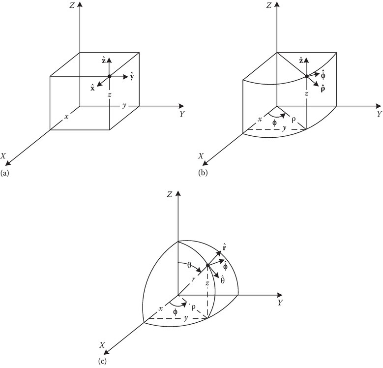
image

FIGURE 1A.1
(a) Rectangular, (b) cylindrical, and (c) spherical coordinate systems.

1A.1.1Rectangular to Cylindrical (and Cylindrical to Rectangular) Transformation

Referring to Figure 1A.1b, the coordinate transformation from rectangular (x, y, z) to cylindrical (ρ, ϕ, z) coordinates is given by

(1A.1)x=ρcosϕ,y=ρsinϕ,z=z.
x=ρcosϕ,y=ρsinϕ,z=z.

In rectangular coordinates, a vector A is written as

(1A.2)A=ˆxAx+ˆyAy+ˆzAz,
A=xˆAx+yˆAy+zˆAz,

where ˆx,ˆy,andˆzxˆ,yˆ,andzˆ are the unit vectors and Ax, Ay, and Az are the components of the vector A in the rectangular coordinate system. We can also write A as

(1A.3)A=ˆρAρ+ˆφAϕ+ˆzAz,
A=ρˆAρ+φˆAϕ+zˆAz,

where ˆρ,ˆφ,andˆzρˆ,φˆ,andzˆ are the unit vectors and Aρ, Aϕ, and Az are the vector components in the cylindrical coordinate system. It can be shown that

(1A.4)ˆx=ˆρcosϕˆφsinϕ,ˆy=ˆρsinϕ+ˆφcosϕ,ˆz=ˆz,
xˆ=ρˆcosϕφˆsinϕ,yˆ=ρˆsinϕ+φˆcosϕ,zˆ=zˆ,

and therefore,

(1A.5)A=(ˆρcosϕˆφsinϕ)Ax+(ˆρsinϕˆφcosϕ)Ay+ˆzAz,A=ˆρ(Axcosϕ+Aysinϕ)ˆφ(Axsinϕ+Aycosϕ)+ˆzAz,
A=(ρˆcosϕφˆsinϕ)Ax+(ρˆsinϕφˆcosϕ)Ay+zˆAz,A=ρˆ(Axcosϕ+Aysinϕ)φˆ(Axsinϕ+Aycosϕ)+zˆAz,

thus

(1A.6)Aρ=Axcosϕ+Aysinϕ,Aϕ=Axsinϕ+Aycosϕ,Az=Az.
Aρ=Axcosϕ+Aysinϕ,Aϕ=Axsinϕ+Aycosϕ,Az=Az.

This can be expressed in the matrix form as

(1A.7)[AρAϕAz]=[cosϕsinϕ0sinϕcosϕ0001][AxAyAz]=[A]rc[AxAyAz],
AρAϕAz=cosϕsinϕ0sinϕcosϕ0001AxAyAz=[A]rcAxAyAz,

where

(1A.8)[A]rc=[cosϕsinϕ0sinϕcosϕ0001]
[A]rc=cosϕsinϕ0sinϕcosϕ0001

is the transformation matrix for rectangular to cylindrical components. Since [A]rc is an orthonormal matrix (its inverse is equal to its transpose), the transformation matrix from cylindrical to rectangular components can be written as

(1A.9)[A]cr=[A]1rc=[A]Trc=[cosϕsinϕ0sinϕcosϕ0001],
[A]cr=[A]1rc=[A]Trc=cosϕsinϕ0sinϕcosϕ0001,
(1A.10)[AxAyAz]=[cosϕsinϕ0sinϕcosϕ0001][AρAϕAz],
AxAyAz=cosϕsinϕ0sinϕcosϕ0001AρAϕAz,
(1A.11)Ax=AρcosϕAϕsinϕ,Ay=Aρsinϕ+Aϕcosϕ,Az=Az.
Ax=AρcosϕAϕsinϕ,Ay=Aρsinϕ+Aϕcosϕ,Az=Az.

1A.1.2Cylindrical to Spherical (and Spherical to Cylindrical) Transformation

From Figure 1A.1c, it can be seen that the cylindrical and spherical coordinates are related by

(1A.12)ρ=rsinθ,z=rcosθ.
ρ=rsinθ,z=rcosθ.

In a manner similar to the previous section, it can be shown that

(1A.13)Ar=Aρsinθ+Azcosθ,Aθ=AρcosθAzsinθ,
Ar=Aρsinθ+Azcosθ,Aθ=AρcosθAzsinθ,

therefore

Aϕ=Aϕ,
Aϕ=Aϕ,

or in matrix notation

(1A.14)[ArAθAϕ]=[sinθ0cosθcosθ0sinθ010][AρAϕAz],
ArAθAϕ=sinθcosθ0001cosθsinθ0AρAϕAz,
(1A.15)[A]cs=[sinθ0cosθcosθ0sinθ010].
[A]cs=sinθcosθ0001cosθsinθ0.

The [A]cs matrix is orthonormal and so its inverse is given by

(1A.16)[A]sc=[A]1cs=[A]Tcs=[sinθcosθ0001cosθsinθ0]
[A]sc=[A]1cs=[A]Tcs=sinθ0cosθcosθ0sinθ010

and the spherical to cylindrical transformation is accomplished by

(1A.17)[AρAϕAz]=[sinθcosθ0001cosθsinθ0][ArAθAϕ],
AρAϕAz=sinθ0cosθcosθ0sinθ010ArAθAϕ,
(1A.18)Aρ=Arsinθ+Aθcosθ,Aϕ=Aϕ,Az=ArcosθAθsinθ.
Aρ=Arsinθ+Aθcosθ,Aϕ=Aϕ,Az=ArcosθAθsinθ.

1A.1.3Rectangular to Spherical (and Spherical to Rectangular) Transformation

From Figure 1A.1c, it can be seen that the rectangular and spherical coordinates are related by

(1A.19)x=rsinθcosϕ,
x=rsinθcosϕ,

or

y=rsinθsinϕ,x=rcosθ,

and the spherical and rectangular components by

(1A.20)Ar=Axsinθcosϕ+Aysinθsinϕ+Azcosθ,Aθ=Axcosθcosϕ+AycosθsinϕAzsinθ,Aϕ=Axsinϕ+Aycosϕ.
Ar=Axsinθcosϕ+Aysinθsinϕ+Azcosθ,Aθ=Axcosθcosϕ+AycosθsinϕAzsinθ,Aϕ=Axsinϕ+Aycosϕ.

In the matrix form,

(1A.21)[ArAθAϕ]=[sinθcosϕsinθsinϕcosθcosθcosϕcosθsinϕsinθsinϕcosϕ0][AxAyAz],
ArAθAϕ=sinθcosϕcosθcosϕsinϕsinθsinϕcosθsinϕcosϕcosθsinθ0AxAyAz,
(1A.22)[A]rs=[sinθcosϕsinθsinϕcosθcosθcosϕcosθsinϕsinθsinϕcosϕ0].
[A]rs=sinθcosϕcosθcosϕsinϕsinθsinϕcosθsinϕcosϕcosθsinθ0.

The [A]rs matrix is orthonormal and so its inverse is given by

(1A.23)[A]sr=[A]1rs=[A]Trs=[sinθcosϕcosθcosϕsinϕsinθsinϕcosθsinϕcosϕcosθsinθ0]
[A]sr=[A]1rs=[A]Trs=sinθcosϕsinθsinϕcosθcosθcosϕcosθsinϕsinθsinϕcosϕ0

and the spherical to rectangular transformation is accomplished by

(1A.24)[AxAyAz]=[sinθcosϕcosθcosϕsinϕsinθsinϕcosθsinϕcosϕcosθsinθ0][ArAθAϕ],
AxAyAz=sinθcosϕsinθsinϕcosθcosθcosϕcosθsinϕsinθsinϕcosϕ0ArAθAϕ,
(1A.25)Ax=Arsinθcosϕ+AθcosθcosϕAϕsinϕ,Ay=Arsinθsinϕ+Aθcosθsinϕ+Aϕcosϕ,Az=ArcosθAθsinθ.
Ax=Arsinθcosϕ+AθcosθcosϕAϕsinϕ,Ay=Arsinθsinϕ+Aθcosθsinϕ+Aϕcosϕ,Az=ArcosθAθsinθ.

1A.2Vector Differential Operators

The differential operators normally include gradient of a scalar (∇ψ), divergence of a vector (∇·A), curl of a vector (∇ × A), Laplacian of a scalar (∇ 2ψ), and Laplacian of a vector (∇ 2A). These will be shown in rectangular, cylindrical, and spherical coordinates as given below.

1A.2.1Rectangular Coordinates

(1A.26)ψ=ˆxψx+ˆyψy+ˆzψz,
ψ=xˆψx+yˆψy+zˆψz,
(1A.27)A=Axx+Ayy+Azz,
A=Axx+Ayy+Azz,
(1A.28)×A=|ˆxˆyˆzxyzAxAyAz|=ˆx(AzyAyz)+ˆy(AxzAzx)+ˆz(AyxAxy),
×A=xˆxAxyˆyAyzˆzAz=xˆ(AzyAyz)+yˆ(AxzAzx)+zˆ(AyxAxy),
(1A.29)ψ=2ψ=2ψx2+2ψy2+2ψz2,
ψ=2ψ=2ψx2+2ψy2+2ψz2,
(1A.30)2A=ˆx2Ax+ˆy2Ay+ˆz2Az.
2A=xˆ2Ax+yˆ2Ay+zˆ2Az.

1A.2.2Cylindrical Coordinates

(1A.31)ψ=ˆρψρ+ˆφ1ρψϕ+ˆzψz,
ψ=ρˆψρ+φˆ1ρψϕ+zˆψz,
(1A.32)A=1ρρ(ρAρ)+1ρAϕϕ+Azz,
A=1ρρ(ρAρ)+1ρAϕϕ+Azz,
(1A.33)×A=ˆρ(1ρAzϕAϕz)+ˆφ(AρzAzρ)+ˆz(1ρ(ρAϕ)ρ1ρAρϕ),
×A=ρˆ(1ρAzϕAϕz)+φˆ(AρzAzρ)+zˆ(1ρ(ρAϕ)ρ1ρAρϕ),
(1A.34)2ψ=1ρρ(ρψρ)+1ρ22ψϕ2+2ψz2,
2ψ=1ρρ(ρψρ)+1ρ22ψϕ2+2ψz2,
(1A.35)2A=(A)××A,
2A=(A)××A,
(1A.36)2A=ˆρ(2Aρρ2+1ρAρρAρρ2+1ρ22Aρϕ22ρ2Aϕϕ+2Aρz2)+ˆφ(2Aϕρ2+1ρAϕρAϕρ2+1ρ22Aϕϕ2+2ρ2Aρϕ+2Aϕz2)+ˆz(2Azρ2+1ρAzρ+1ρ22Azϕ2+2Azz2).
2A=ρˆ(2Aρρ2+1ρAρρAρρ2+1ρ22Aρϕ22ρ2Aϕϕ+2Aρz2)+φˆ(2Aϕρ2+1ρAϕρAϕρ2+1ρ22Aϕϕ2+2ρ2Aρϕ+2Aϕz2)+zˆ(2Azρ2+1ρAzρ+1ρ22Azϕ2+2Azz2).

1A.2.3Spherical Coordinates

(1A.37)ψ=ˆrψr+ˆθ1rψθ+ˆφ1rsinθψϕ,
(1A.38)A=1r2r(r2Ar)+1rsinθθ(sinθAθ)+1rsinθAϕϕ,
(1A.39)×A=ˆrrsinθ(θ(sinθAϕ)Aθϕ)+ˆθr(1sinθArϕr(rAϕ))+ˆφr(r(rAθ)Arθ),
(1A.40)2ψ=1r2r(r2ψr)+1r2sinθθ(sinθψθ)+1r2sin2θ2ψϕ2,
(1A.41)2A=(A)××A,
(1A.42)2A=ˆr(2Arr2+2rArr2r2Ar+1r22Arθ2+cotθr2Arθ+1r2sin2θ2Arϕ22r2Aθθ2cotθr2Aθ2r2sinθAϕϕ)+ˆθ(2Aθr2+2rAθrAθr2sin2θ+1r22Aθθ2+cotθr2Aθθ+1r2sin2θ2Aθϕ2+2r2Arθ2cotθr2sinθAϕϕ)+ˆφ(2Aϕr2+2rAϕr1r2sin2θAϕ+1r22Aϕθ2+cotθr2Aϕθ+1r2sin2θ2Aϕϕ2+2r2sinθArϕ+2cotθr2sinθAθϕ).

1A.3Vector Identities

1A.3.1Addition and Multiplication

(1A.43)AA=|A|2=A2,
(1A.44)AA*=|A|2=A2,
(1A.45)A+B=B+A,
(1A.46)AB=BA,
(1A.47)A×B=B×A,
(1A.48)(A+B)C=AC+BC,
(1A.49)(A+B)×C=A×C+B×C,
(1A.50)AB×C=BC×A=CA×B,
(1A.51)A×(B×C)=(AC)B(AB)C,
(1A.52)(A×B)(C×D)=AB×(C×D)=A(BDCBCD)=(AC)(BD)(AD)(BC),
(1A.53)(A×B)×(C×D)=(A×BD)C(A×BC)D.

1A.3.2Differentiation

(1A.54)(×A)=0,
(1A.55)×ψ=0,
(1A.56)(ϕ+ψ)=ϕ+ψ,
(1A.57)(ϕψ)=ϕψ+ψϕ,
(1A.58)(A+B)=A+B,
(1A.59)×(A+B)=×A+×B,
(1A.60)(ψA)=Aψ+ψA,
(1A.61)×(ψA)=ψ×A+ψ×A,
(1A.62)(AB)=(A)B+(B)A+A×(×B)+B×(×A),
(1A.63)(A×B)=B×AA×B,
(1A.64)×(A×B)=ABBA+(B)A(A)B,
(1A.65)××A=(A)2A.

1A.3.3Integration

(1A.66)CAdl=S(×A)ds(Stokes'theorem),
(1A.67)SAds=V(A)dv(Divergencetheorem),
(1A.68)S(ˆn×A)ds=V(×A)dv,
(1A.69)Sψds=Vψdv,
(1A.70)Cψdl=Sˆn×ψds.

Reference

  1. 1.Balanis, C. A., Advanced Engineering Electromagnetics, Wiley, New York, 1989.
..................Content has been hidden....................

You can't read the all page of ebook, please click here login for view all page.
Reset
52.14.240.178