Search in book...
Toggle Font Controls
Create new playlist

Name your new playlist

Playlist description (optional)
Sign In

Email address

Password

Forgot Password?

or

Continue with Facebook

Continue with Google
Sign Up

Full Name

Email address

Confirm Email Address

Password

or

Continue with Facebook

Continue with Google

Appendix 9A: Backscatter from a Plasma Plume due to Excitation of Surface Waves*

Appendix 9A: Backscatter from a Plasma Plume due to Excitation of Surface Waves *

Dikshitulu K. Kalluri

9A.1Introduction

Dr. Keith Groves, my focal point at PL/GP for the Air Force Office of Scientific Research Summer Faculty Research Program (1994), suggested me to investigate the following problem: Experiments conducted by Air Force Laboratories showed that considerable unexpected electromagnetic backscatter from a plasma plume is occurring in a certain intermediate frequency band.

Figures 9A.1 and 9A.2 show the electron density and collision frequency numbers in the plasma plume. The plume is a cylindrical inhomogeneous lossy plasma column. The maximum electron density N_0m on the axis (r = 0) is 3E13 (#/cm³) corresponding to angular plasma frequency (note: for convenience, the computer notation Exx = 10^XX will be used occasionally):

(9A.1)

ω_{pm} = \sqrt{\frac{N_{0 m} e^{2}}{m ε_{0}}} = 3 \times 10^{11} (rad / s)

$ω_{pm} = \sqrt{\frac{N_{0 m} e^{2}}{m ε_{0}}} = 3 \times 10^{11} (rad / s)$

and f_pm = ω_pm/2π = 47.75 GHz. Here m and e are the mass and absolute value of the charge of an electron, respectively, and ε₀ = 8.854E−12 (F/m) is the permittivity of the free space. The collision frequency (ν) also varies with r ranging in value from 6E11 to 1E11 (rad/s). Scattering of an electromagnetic wave, in the frequency range of f = 50 MHz to 10 GHz, by such an inhomogeneous and lossy plasma plume is the object of this investigation.

FIGURE 9A.1
Electron density of the plasma plume. (Reprinted from Final Report Summer Faculty Research Program, *Air Force Office of Scientific Research*, Report Number A669853, 38, 1994. With permission.)

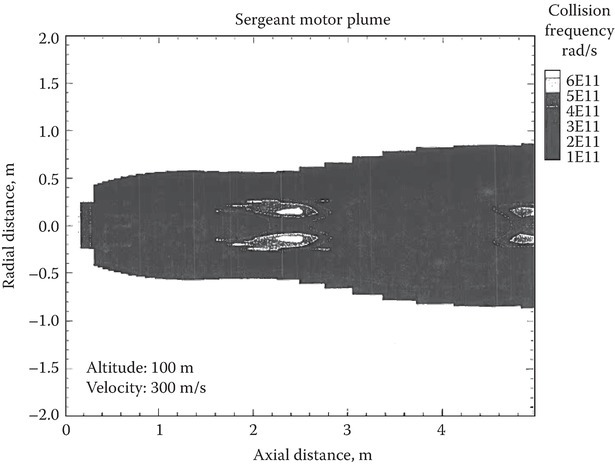
FIGURE 9A.2
Collision frequency of the plasma plume. (Reprinted from Final Report Summer Faculty Research Program, *Air Force Office of Scientific Research*, Report Number A669853, 38, 1994. With permission.)

9A.2Problem Classification Based on Plasma Parameters

Plasma radius a is of the order of 0.5 m; the normalized value a/λ_pm = af_pm/c = 83.3. In this sense, the column may be classified as thick.

Here c is the velocity of light = 3 × 10⁸ m/s and λ_pm is the free space wavelength of the corresponding plasma frequency.
The normalized value a/λ = af/c varies from 8.3 × 10⁻² to 16.67 as f varies from 50 MHz to 10 GHz, respectively.
The collision frequency (ν) is quite high and is of the order of plasma frequency on the axis. The plasma has to be classified as highly collisional.
The outer layer around r = a has a turbulent character.
Apart from the outer layer, the rest of the column behaves like an overdense plasma (good conductor), for the frequency range 50 MHz to 10 GHz.
The fact that r > a is free space and r < a, overdense plasma that behaves like a conductor suggests that the column is capable of supporting TM surface waves. The outer edge near r = a, being turbulent, behaves like a rough surface [1] for f < f_p.

The author of this report (henceforth will be referred to as the author) is strongly influenced by his experience with the study of surface plasmons at optical frequencies and wondered whether their excitation in this case will result in backscatter. However, before launching a full investigation into this aspect, the author wanted to understand the absorption of the high-frequency electromagnetic radiation by the highly collisional inhomogeneous plasma. This aspect is discussed in the following section.

9A.3Absorption of TM Wave

The problem of the absorption of the electromagnetic wave by the highly collisional plasma column is studied by modeling the column as an inhomogeneous lossy plasma slab of width d = 2a. Figure 9A.3 shows this model, where the inhomogeneity is mathematically modeled, for illustrative purposes, by a trigonometric function given below:

(9A.2)

ω_{p} (z) = ω_{pm} {(\frac{sin π z}{d})}^{m / 2} .

$ω_{p} (z) = ω_{pm} {(\frac{sin π z}{d})}^{m / 2} .$

FIGURE 9A.3
Mathematical model for the inhomogeneity. (Reprinted from Final Report Summer Faculty Research Program, *Air Force Office of Scientific Research*, Report Number A669853, 38, 1994. With permission.)

By changing the value of m, the profile may be altered to fit the experimental profile approximately.

In the region 0 < z < d, the equations satisfied by the time-harmonic fields are given below:

(9A.3)

\bar{\nabla} \times \bar{E} = - j ω μ_{0} \bar{H},

$\bar{\nabla} \times \bar{E} = - j ω μ_{0} \bar{H},$

(9A.4)

\bar{\nabla} \times \bar{H} = - N_{0} e \bar{v} + j ω ε_{0} \bar{E},

$\bar{\nabla} \times \bar{H} = - N_{0} e \bar{v} + j ω ε_{0} \bar{E},$

(9A.5)

j ω m \bar{v} = - e \bar{E} - m ν \bar{v} .

$j ω m \bar{v} = - e \bar{E} - m ν \bar{v} .$

Here E, H, and v are the electric, the magnetic, and the velocity fields, respectively. The other symbols have the usual meaning. Assuming the field quantities vary as

(9A.6)

F (x, z, t) = F (z) e^{j (ω t - S x)} .

$F (x, z, t) = F (z) e^{j (ω t - S x)} .$

The first-order-coupled differential equations satisfied by the state variables E_x and (η₀ H_y) of a TM wave are obtained:

(9A.7)

- \frac{1}{j k_{0}} \frac{d E_{x}}{d z} = \frac{C^{2} - X / U}{1 - X / U} (η_{0} H_{y}),

$- \frac{1}{j k_{0}} \frac{d E_{x}}{d z} = \frac{C^{2} - X / U}{1 - X / U} (η_{0} H_{y}),$

(9A.8)

- \frac{1}{j k_{0}} \frac{d (η_{0} H_{y})}{d z} = (1 - X / U) E_{x} .

$- \frac{1}{j k_{0}} \frac{d (η_{0} H_{y})}{d z} = (1 - X / U) E_{x} .$

Here S = sin θ, C = cos θ, θ is the angle of incidence (angle with z-axis), k₀ = ω/c, η₀ is the characteristic impedance of free space = (μ₀/ε₀)^1/2 = 120π and the symbols X and U (notation used in magnetoionic theory) are

(9A.9a)

X (z) = {(\frac{ω_{p} (z)}{ω})}^{2},

$X (z) = {(\frac{ω_{p} (z)}{ω})}^{2},$

(9A.9b)

U = 1 - j Z, Z (z) = \frac{ν (z)}{ω} .

$U = 1 - j Z, Z (z) = \frac{ν (z)}{ω} .$

The following numerical method is devised to obtain the absorption coefficient.

Assume a suitable arbitrary complex value K_X for E_X at z = d, that is, $E_{X} (d) = K_{X} = E_{X}^{T} .$ $E_{X} (d) = K_{X} = E_{X}^{T} .$ It follows that (η₀ H_y) at z = d is K_X/C.
Starting with these initial values, solve, numerically the first-order-coupled differential equations (9A.7) and (9A.8) by integrating downwards and obtain E_X(0) = a_X and η₀H_y(0) = b_y.
Calculate the reflection and transmission coefficients:

(9A.10) $R_{11} = \frac{E_{x}^{R}}{E_{x}^{I}} = \frac{a_{x} - C b_{y}}{a_{x} + C b_{y}},$ $R_{11} = \frac{E_{x}^{R}}{E_{x}^{I}} = \frac{a_{x} - C b_{y}}{a_{x} + C b_{y}},$

(9A.11) $|T_{11}| = |\frac{E_{x}^{T}}{E_{x}^{I}}| = |\frac{2 K_{x}}{a_{x} + C b_{y}}| .$ $|T_{11}| = |\frac{E_{x}^{T}}{E_{x}^{I}}| = |\frac{2 K_{x}}{a_{x} + C b_{y}}| .$

Here the superscripts I, R, and T refer to incident, reflected, and transmitted fields, respectively. The subscript 11 refers to the parallel (TM) polarization of the incident wave.
Calculate the absorption coefficient:

(9A.12) $A = 1 - ρ - τ = 1 - {|R_{11}|}^{2} - {|T_{11}|}^{2},$ $A = 1 - ρ - τ = 1 - {|R_{11}|}^{2} - {|T_{11}|}^{2},$

where ρ and τ are power reflection and transmission coefficients.

Figure 9A.4a through c are graphs for ρ, τ, and A versus f for an angle of incidence of 60°, respectively. Here ν is assumed constant and is equal to 3E11 (rad/s). From these graphs, it is clear that absorption increases with frequency. This result may be qualitatively explained by noting that the depth of penetration of the source wave increases with frequency since the value of z at which ω_p(z) = ω increases with increase of f. In passing, it may be noted that a pseudo-Brewster angle exists for the TM case under consideration and shown in Figure 9A.5.

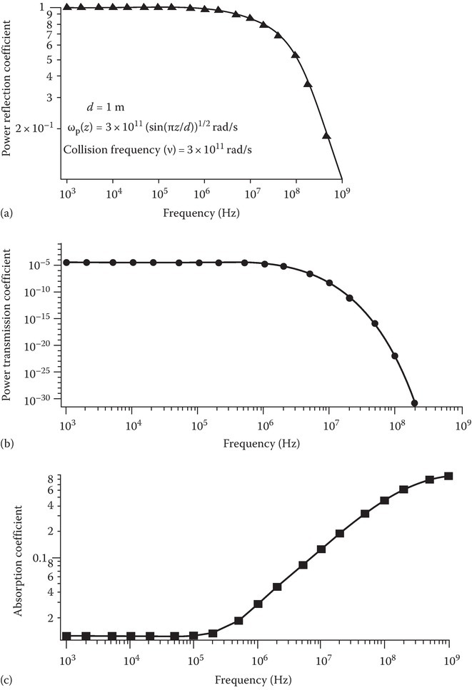
FIGURE 9A.4
Frequency dependence of various power coefficients: (a) reflection, (b) transmission, and (c) absorption angle of incidence is 60°. (Reprinted from Final Report Summer Faculty Research Program, *Air Force Office of Scientific Research*, Report Number A669853, 38, 1994. With permission.)

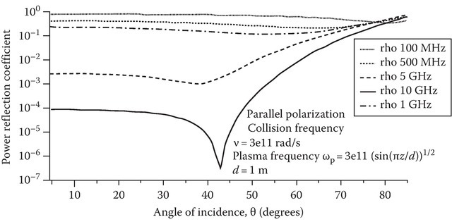
FIGURE 9A.5
Power reflection coefficient vs. angle of incidence. (Reprinted from Final Report Summer Faculty Research Program, *Air Force Office of Scientific Research*, Report Number A669853, 38, 1994. With permission.)

In conclusion, a theory based on only specular reflection and associated physics assumed above does not perhaps explain the increased backscatter in an intermediate frequency range. This led us to consider incorporating new physics into our model.

Turbulence present in the outer layers perhaps plays some part. Since for the frequency range under consideration, the plasma is overdense, the turbulent layer is modeled as a rough surface. The inner layers behave like a gaseous conductor. These thoughts led the author to consider the aspect of surface wave excitation.

9A.4Review of Surface Waves

A surface wave [2,3] propagates along the surface x = 0 (see Figure 9A.6), with a phase velocity V_ph = ω/k_z. Its fields attenuate for |x| > 0. An interface between two dielectrics can support such a wave provided their dielectric constants are of opposite sign and ε_r1 < −ε_r2. If medium 2 is the free space and medium 1 is a plasma whose plasma frequency is such that $ε_{r 1} = (1 - ω_{p}^{2} / ω^{2}) < - 1,$ $ε_{r 1} = (1 - ω_{p}^{2} / ω^{2}) < - 1,$ the conditions for the support of a surface wave at the interface are satisfied. Such a surface wave is called surface plasmon. For optical frequencies, medium 1 is a metal which behaves like a plasma with negative dielectric constant.

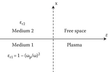
FIGURE 9A.6
Free space-plasma interface. (Reprinted from Final Report Summer Faculty Research Program, *Air Force Office of Scientific Research*, Report Number A669853, 38, 1994. With permission.)

However, an electromagnetic wave in free space incident at any angle on the interface cannot excite the surface wave since the dispersion characteristic of the surface wave (k_z vs. ω) lies to the right of the light line (see Figure 9A.7b for an illustrative graph in which β is the real part of k_z). In optics, the required additional ∆k_z is obtained by using a ATR coupler or a grating coupler or a rough surface.

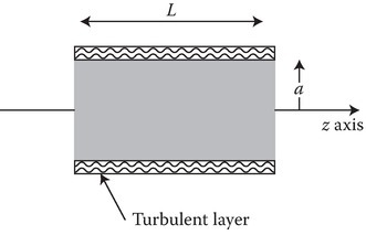
FIGURE 9A.7
Plasma with a turbulent layer. (Reprinted from Final Report Summer Faculty Research Program, *Air Force Office of Scientific Research*, Report Number A669853, 38, 1994. With permission.)

9A.5Excitation of Surface Waves on Plasma Plume

From the material presented in Sections 9A.2 and 9A.4, it is clear that conditions exist for the excitation of a surface wave on the surface of the plasma plume. In this section, the equations needed to obtain the dispersion relation [3,4] of the surface plasmons are discussed (refer to Figure 9A.7).

Plasma region (0 < r < a):

(9A.13)

ε_{p} (r) = 1 - \frac{ω_{p}^{2} (r)}{ω (ω - j ν)} .

$ε_{p} (r) = 1 - \frac{ω_{p}^{2} (r)}{ω (ω - j ν)} .$

Let

(9A.14)

E_{z}^{p} (r, ϕ, z, t) = A G (r) e^{j (ω t - k_{z} z)},

$E_{z}^{p} (r, ϕ, z, t) = A G (r) e^{j (ω t - k_{z} z)},$

where

(9A.15)

- k_{tp}^{2} (r) + k_{z}^{2} = k_{0}^{2} ε_{p} (r), k_{0} = \frac{ω}{c}

$- k_{tp}^{2} (r) + k_{z}^{2} = k_{0}^{2} ε_{p} (r), k_{0} = \frac{ω}{c}$

and G(r) satisfies the differential equation:

(9A.16)

\frac{d^{2} G}{d r^{2}} + [\frac{1}{r} + \frac{k_{z}^{2}}{k_{tp}^{2} (r)} \frac{d ε_{p} /d r}{ε_{p} (r)}] \frac{d G}{d r} - k_{tp}^{2} (r) G = 0.

$\frac{d^{2} G}{d r^{2}} + [\frac{1}{r} + \frac{k_{z}^{2}}{k_{tp}^{2} (r)} \frac{d ε_{p} /d r}{ε_{p} (r)}] \frac{d G}{d r} - k_{tp}^{2} (r) G = 0.$

Other field components of this TM wave can be expressed in terms of the z-component of the electric field.

(9A.17a)

E_{r}^{p} = - \frac{j}{k_{t 0}^{2}} k_{z} \frac{\partial E_{z}^{p}}{\partial r},

$E_{r}^{p} = - \frac{j}{k_{t 0}^{2}} k_{z} \frac{\partial E_{z}^{p}}{\partial r},$

(9A.17b)

H_{ϕ}^{p} = - \frac{j}{k_{t 0}^{2}} ω ε_{0} ε_{p} \frac{\partial E_{z}^{p}}{\partial r},

$H_{ϕ}^{p} = - \frac{j}{k_{t 0}^{2}} ω ε_{0} ε_{p} \frac{\partial E_{z}^{p}}{\partial r},$

(9A.17c)

Z_{TM}^{z} = \frac{E_{r}}{H_{ϕ}} = \frac{k_{z}}{ω ε_{0} ε_{p}} .

$Z_{TM}^{z} = \frac{E_{r}}{H_{ϕ}} = \frac{k_{z}}{ω ε_{0} ε_{p}} .$

Free space region (a < r < ∞):

(9A.18)

\frac{d^{2} E_{z}^{0}}{d r^{2}} + \frac{1}{r} \frac{d E_{z}^{0}}{d r} - k_{t 0}^{2} E_{z}^{0} = 0,

$\frac{d^{2} E_{z}^{0}}{d r^{2}} + \frac{1}{r} \frac{d E_{z}^{0}}{d r} - k_{t 0}^{2} E_{z}^{0} = 0,$

(9A.19)

- k_{t 0}^{2} (r) + k_{z}^{2} = k_{0}^{2},

$- k_{t 0}^{2} (r) + k_{z}^{2} = k_{0}^{2},$

(9A.20)

E_{z}^{0} (r, ϕ, z, t) = B K_{0} (k_{t 0} r) e^{j (ω t - k_{z} z)},

$E_{z}^{0} (r, ϕ, z, t) = B K_{0} (k_{t 0} r) e^{j (ω t - k_{z} z)},$

(9A.21a)

E_{r}^{0} (r, ϕ, z, t) = j B \frac{k_{z}}{k_{t 0}} K_{1} (k_{t 0} r) e^{j (ω t - k_{z} z)},

$E_{r}^{0} (r, ϕ, z, t) = j B \frac{k_{z}}{k_{t 0}} K_{1} (k_{t 0} r) e^{j (ω t - k_{z} z)},$

(9A.21b)

H_{ϕ}^{0} (r, ϕ, z, t) = \frac{j B}{k_{t 0}} ω ε_{0} K_{1} (k_{t 0} r) e^{j (ω t - k_{z} z)} .

$H_{ϕ}^{0} (r, ϕ, z, t) = \frac{j B}{k_{t 0}} ω ε_{0} K_{1} (k_{t 0} r) e^{j (ω t - k_{z} z)} .$

Here K₀ and K₁ are the modified Bessel functions of the second kind [5]. From the boundary conditions of continuity of E_z and H_ϕ at r = a, the following dispersion relation is obtained:

(9A.22)

\frac{k_{tp}^{2} (a)}{ε_{p} (a)} \frac{G (a)}{G^{'} (a)} + k_{t 0} \frac{K_{0} (k_{t 0} a)}{K_{1} (k_{t 0} a)} = 0.

$\frac{k_{tp}^{2} (a)}{ε_{p} (a)} \frac{G (a)}{G^{'} (a)} + k_{t 0} \frac{K_{0} (k_{t 0} a)}{K_{1} (k_{t 0} a)} = 0.$

In these equations while ω is real, k_z and several other quantities are complex and the complex mode is to be used for computations. In particular, let us denote

(9A.23)

k_{z} = β - j α,

$k_{z} = β - j α,$

where β the phase constant and α the attenuation constant are real. The propagation velocity of the surface wave is given by

(9A.24)

V_{ph} = \frac{ω}{β} .

$V_{ph} = \frac{ω}{β} .$

9A.6Numerical Method for Obtaining the Dispersion Relation

The above equations are used to compute the complex value of k_z for a given real value of ω. Numerical mode of the software Mathematica is used. The method consists of iterating between the two steps outlined below till convergence is obtained:

Step 1: Starting with a guessed value for k_z, the differential equation (9A.16) for G is numerically solved, with the initial conditions G(0) = 0 and G′(0) = 0. The singularity at r = 0 has to be handled with care. Thus, the values of G(a) and G′(a) are obtained.
Step 2: The dispersion relation which is a nonlinear algebraic equation is now solved for k_z.

Since the cylinder is thick, it is possible that for some values of ω, both G(a) and G′(a) are large though their ratio is not large. To cover this aspect, an alternative numerical method is also developed. The second-order differential equation for G is converted into a first-order nonlinear differential equation by defining a new variable Y = G′/G, which has the initial condition Y = 0:

(9A.25)

\frac{d Y}{d r} + [\frac{1}{r} + \frac{k_{z}^{2}}{k_{tp}^{2} (r)} \frac{d ε_{p} / d r}{ε_{p} (r)}] Y + Y^{2} - k_{tp}^{2} (r) = 0.

$\frac{d Y}{d r} + [\frac{1}{r} + \frac{k_{z}^{2}}{k_{tp}^{2} (r)} \frac{d ε_{p} / d r}{ε_{p} (r)}] Y + Y^{2} - k_{tp}^{2} (r) = 0.$

Once again the singularity at r = 0 has to be handled with care.

9A.7Back Scatter

The surface traveling wave on the plasma plume is analogous to a current wave along thin-wire antennas [6] in the end-fire mode. It travels with a velocity close to that of light. The far-radiated field

(9A.26)

E_{r} = - A j k_{0} L sin θ_{1} \frac{sin [(1 / 2 p) k_{0} L (1 - p cos θ_{1})]}{(1 / 2 p) k_{0} L (1 - p cos θ_{1})},

$E_{r} = - A j k_{0} L sin θ_{1} \frac{sin [(1 / 2 p) k_{0} L (1 - p cos θ_{1})]}{(1 / 2 p) k_{0} L (1 - p cos θ_{1})},$

where A is a constant with respect to θ₁ and L, θ₁ the angle of the point of observation away from the axis of the plume, and p the propagation velocity divided by c. p is close but slightly less than 1. The surface wave traveling a distance L along the axis is reflected when it encounters a spatial discontinuity in the properties of the medium at z = L. It is the reflected wave that gives rise to the backscatter. Figure 9A.8 gives a qualitative explanation [6] for the backscatter. For p close to 1, the first maximum in the pattern [5] occurs at

(9A.27)

θ_{1} = 49.35 \sqrt{\frac{λ}{L}} (deg) .

$θ_{1} = 49.35 \sqrt{\frac{λ}{L}} (deg) .$

FIGURE 9A.8
Reflected wave giving rise to the back scatter. (Reprinted from Final Report Summer Faculty Research Program, *Air Force Office of Scientific Research*, Report Number A669853, 38, 1994. With permission.)

9A.8Sample Calculation

The electron density is assumed to be varying radially as a Bessel function of the first kind of zero order. Consequently, the square of the plasma frequency is given by

(9A.28)

ω_{p}^{2} (r) = ω_{pm}^{2} J_{0} (μ \frac{r}{a}) .

$ω_{p}^{2} (r) = ω_{pm}^{2} J_{0} (μ \frac{r}{a}) .$

If μ = 0, then we have the homogeneous case and if μ = 2.405 the plasma density at the edge r = a is zero. For the sample calculation, we chose μ = 2.1. Thus,

(9A.29)

ω_{p} (a) = ω_{pm} \sqrt{J_{0} (2.1)} = 0.4082 ω_{pm} .

$ω_{p} (a) = ω_{pm} \sqrt{J_{0} (2.1)} = 0.4082 ω_{pm} .$

Choosing further ω_pm = 3E11 (rad/s), plasma frequency f_p(a) = 19.51 GHz.

For the purpose of illustration, let the turbulent layer be described by 0.4 < r < 0.5, thus a = 0.4 m. The collision frequency ν is taken to be 1.E11 (rad/m) which is the value in the outer layers. Using these parameters α versus f and β versus f are obtained numerically as described in Section 9A.6. Figure 9A.9 shows these results. The value of L = 1 m is assumed where from Figure 9A.2, there appears to be a discontinuity in the properties of the medium. For an illustrative value of f = 600 MHz, λ = 0.5 m and from Equation 9A.27, θ₁ = 34.9°. The line to the left of the dispersion curve marked as surface wave on plasma column is the light line for an EM wave in free space incident at 34.9° with the axis. This curve is a straight line described by the equation:

(9A.30)

k_{z 0} = k_{0} cos 34.9 ° .

$k_{z 0} = k_{0} cos 34.9 ° .$

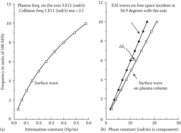
FIGURE 9A.9
Sample calculation: (a) attenuation constant and (b) phase constant. (Reprinted from Final Report Summer Faculty Research Program, *Air Force Office of Scientific Research*, Report Number A669853, 38, 1994. With permission.)

The horizontal line marked as ∆k_z = 2.29 is proportional to the z-component of the momentum (in the language of photonics) that is supplied by the turbulent rough surface. Superposition of the spectrum of plasma turbulence will lead to the frequency band of the surface waves that can be excited. Figure 9A.9a permits us to calculate the attenuation suffered by the surface wave in traveling a distance L before it reaches the point of discontinuity. At 600 MHz, α = 0.26119 and exp(−2αL) = 59.3%. Thus, 60% of power is still in tact for backscattering. All the numbers were obtained assuming p is nearly equal to 1 and this may be verified by calculating ω/β at f = 600 MHz. This gives a propagation velocity of 2.9767e8 m/s confirming p ≈ 1.

9A.9Results and Conclusions

Based on the results obtained so far, the following observations can be made with reference to the various parameters.

Effect of frequency: At low frequencies, the radiation field given in Equation 9A.26, which is inversely proportional to λ, is weak. At high frequencies, the attenuation constant is high and the surface wave is dissipated before it reaches the discontinuity and therefore the backscattering is weak.

Effect of L: As L increases, the radiation field increases as seen from Equation 9A.26 but the aspect angle θ₁ decreases, ∆kz decreases facilitating easier excitation of the surface waves. There is no change in α or β. However, the wave attenuation increases because of the increase in L. Perhaps, the center of the frequency band of significant backscatter moves toward higher frequencies as L increases.

Effect of polarization: The model assumed TM waves, since surface plasmons can be excited only when the wave electric field has a z-component.

9A.10Scope for Future Work

A theory based on the excitation of surface waves on a plasma plume is constructed to offer a plausible explanation for increased backscatter in an intermediate frequency band. Sample calculations are made based on a simple model and approximate data. The theory will be improved and more accurate calculations will be made based on some more experimental data. Spectrum of the turbulent plasma will be incorporated into the model when the experimental data on this aspect becomes available. The author intends to submit summer research extension proposal to complete this work.

References

1.Hochstin, A. R. and Martens, C. P., Proceedings of Symposium on Turbulence of Fluids and Plasmas, Polytechnic Press, New York, 1968, p. 187.
2.Raether, H., Surface Plasmons, Springer, Berlin, Germany, 1988.
3.Boardman, A. D. (Ed.), Electromagnetic Surface Modes, Wiley, New York, 1982.
4.Zethoff, M. and Kortshagen, U., J. Phys. D: Appl. Phys., 25, 187, 1992.
5.Abramowitz, M. and Stegun, I. A. (Eds.), Handbook of Mathematical Functions, Dover Publications, New York, 1965.
6.Knott, E. F., Shaeffer, J. F., and Tuley, M. T., Radar Cross Section, Artech House, Boston, MA, 1985, p. 148.

..................Content has been hidden....................

You can't read the all page of ebook, please click here login for view all page.